Table of Contents

• 1  Learning objectives

• 2  Introduction

• 3  The context module (repeated from 10-pandas1)

• 4  Reading the processed data

• 5  Metadata is data about data

• 6  Read weather_YVR.csv into a dataframe

  • 6.1  Handling missing data

• 7  Use apply to tag the 29,190 days with their season

  • 7.1  creating a new column with apply

• 8  Grouping the data by season

  • 8.1  Use a dictionary comprehension put the dataframes into a dictionary

• 9  Fitting the distributions

  • 9.1  Daily average temperature

    • 9.1.1  Missing values again

  • 9.2  Daily average total precipitation

• 10  Saving the fit parameters

• 11  Grouping by decade

• 12  Finding the median temperature

• 13  Assignment

Analyzing precip and temperature data

Learning objectives

1. Document your project data by capturing important information as metadata in a json file

2. Use the groupby method for a pandas dataframe to group observations by season

3. Find the probability density function (histogram) of temperature and precipitation data and determine possible statistical models (normal distribution, exponential distribution) that best describe the variation in the data

4. Find best fit parameters for statistical models that describe the precipitation and temperature data, assuming that temperature and precipitation are independent of each other.

5. Use groupby to find the median temperature for each decade and each season and determine whether the seasonal temperatures have increased at YVR since the 1930’s

Introduction

We have about 30,000 days worth of YVR precipitation and temperature data generated by the 10-pandas1, 10-pandas2, and 10-pandas3 notebooks, these gave you a new csv file: data/processed/weather_YVR.csv. We will use that data set to estimate statistical distributions that could produce realistic simulated rainfall and temperature inputs to a model. It makes use of several new python modules/methods:

1. The context module: We will write a new module called context.py that will be used to locate folders and libraries associated with a project, such as weather_YVR.csv.

2. The json module. This reads and writes files written in “javascript object notation” i.e. json. We will use it to save “metadata” or data about our data.

3. pandas.DataFrame.groupby We will use groupby to split the dataframe into 4 seasons, each corresponding to 3 months of the year: winter (month initials djf), spring (mam), summer (jja), and fall (son). This is the tip of the iceberg of what you can do with pandas split/apply/combine functions. For more examples see the Python Data Science Handbook

4. The scipy.stats module. As you will see below, the temperature data is best fit with a a Gaussian (normal) distribution using the norm.fit:

   • scipy.stats.norm.fit

   Precipitation, on the other hand, follows an exponential distribution, which can be fit with:

   • scipy.stats.expon.fit

import json

import context
import pandas as pd
import scipy.stats as st
from matplotlib import pyplot as plt
import pprint
import numpy as np

in context.py, found /Users/phil/repos/eosc213_students/notebooks/pandas/data/processed

The context module (repeated from 10-pandas1)

As your project grows more complicated, it’s good to have a central module that keeps track of important files and sets your scripts up so that they can import functions and classes from you modules. If you were planning to distribute your project using conda, then you would need to write an installation script, which is a fair amount of work. At this stage, it’s easier and more flexible to store that information in a file that travels along with your notebook. By convention, this file is called: context.py

Clicking on that link shows you the source – the code is executed when you do import context and does the following:

1. Defines Path objects that give the location of the raw and processed data folders

2. Puts the notebooks/pandas folder on python’s list of places to look for library modules (sys.path). We will use this when we start extracting code from notebooks into libraries

#
# Here is the path to the processed csv file
#
print(context.processed_dir)

/Users/phil/repos/eosc213_students/notebooks/pandas/data/processed

Reading the processed data

The next cell uses “globbing” to find every csv file in all folders below data/processed. (See this optional tutorial for more information).

yvr_files = list(context.processed_dir.glob("**/*YVR*csv"))
print(f"yvr files: \n{pprint.pformat(yvr_files)}")

yvr files:
[PosixPath('/Users/phil/repos/eosc213_students/notebooks/pandas/data/processed/weather_daily_YVR_1938-2017_all.csv'),
 PosixPath('/Users/phil/repos/eosc213_students/notebooks/pandas/data/processed/weather_daily_YVR_1938-2019_all.csv'),
 PosixPath('/Users/phil/repos/eosc213_students/notebooks/pandas/data/processed/weather_YVR.csv')]

yvr_file = context.processed_dir / "weather_YVR.csv"

Metadata is data about data

Since we care about this dataset, it’s a good idea to save details for future reference. We can’t put this kind of information into a csv file, but there are many file formats that can store this type of descriptive metadata – one of the most popular is json. In the next cell we write the data into a nested dictionary called meta_dict, and dump that information into a new json file called metadata.json

meta_data = dict()

file_info = dict()
file_info["written_by"] = "10-pandas3-process-daily-data.ipynb"
file_info["contact"] = "paustin@eoas.ubc.ca"
file_info[
    "description"
] = "EC canada YVR data downloaded by 10-pandas2-download-daily-data.ipynb"

meta_data["weather_daily_YVR_1938-2017_all.csv"] = file_info

file_info = dict()
file_info["written_by"] = "10-pandas3-process-daily-data.ipynb"
file_info["contact"] = "paustin@eoas.ubc.ca"
file_info[
    "description"
] = "Reduced YVR data subsetted by 10-pandas3-process-daily-data.ipynb"

meta_data["weather_YVR.csv"] = file_info

history_file = context.processed_dir / "history_metadata.json"
with open(history_file, "w") as f:
    json.dump(meta_data, f, indent=4)

Take a minute and look at history_metadata.json with jupyter to see how the metadata is written out.

Read weather_YVR.csv into a dataframe

Here’s the dataframe produced by 10-pandas3

yvr_df = pd.read_csv(yvr_file)
print(f"there are {len(yvr_df)} days in the dataframe")
yvr_df.head()

there are 29632 days in the dataframe

	Date	Year	Month	Day	T_mean (C)	T_high (C)	T_low (C)	Rain (mm)	Snow (cm)	Total Precip (mm)
0	1938-01-01	1938	1	1	4.4	9.4	-0.6	NaN	NaN	0.3
1	1938-01-02	1938	1	2	4.5	7.2	1.7	NaN	NaN	0.5
2	1938-01-03	1938	1	3	1.7	7.2	-3.9	0.0	0.0	0.0
3	1938-01-04	1938	1	4	2.2	7.2	-2.8	0.0	0.0	0.0
4	1938-01-05	1938	1	5	2.2	7.2	-2.8	0.0	0.0	0.0

Handling missing data

What should we do about missing vlaues like the Rain and Snow totals for Jan./Feb. 1938? This is a judgement call – we could through away the whole row, or do something more complicated like masking the missing values in calculations where they are referenced. For this notebook we’ll fill the NaNs with zeros – not a great idea since 0 is an actual temperature, but we can see if that makes a difference later

yvr_df_zeros=yvr_df.fillna(0.)

Use apply to tag the 29,190 days with their season

We know that the seasons are quite different, and if we are interested in generating daily data we have to take that into account. In the next cell we set up a lookup table (dictionary) called season_table that maps the month number to one of four seasons. With this table we can write a function called find_season that takes a row of the dataframe and returns the season for that row

season_table = dict()
for i in range(12):
    m = i + 1
    if m in [12, 1, 2]:
        # winter
        season_table[m] = "djf"
    elif m in [3, 4, 5]:
        # spring
        season_table[m] = "mam"
    elif m in [6, 7, 8]:
        # summer
        season_table[m] = "jja"
    else:
        # fall
        season_table[m] = "son"


def find_season(row, season_table):
    month = row["Month"]
    return season_table[month]

creating a new column with apply

One of the most useful pandas dataframe methods is apply. This method has lots of bells and whistles, all we need here is to apply the find_season function to every row of the dataframe, which means that we want to return a new column with the same number of rows as the other columns. We do that by tell apply that we want to return axis=1 (rows are axis=0)

season = yvr_df.apply(find_season, args=(season_table,), axis=1)

Now add that column to the dataframe

yvr_df["season"] = season
yvr_df.head()

	Date	Year	Month	Day	T_mean (C)	T_high (C)	T_low (C)	Rain (mm)	Snow (cm)	Total Precip (mm)	season
0	1938-01-01	1938	1	1	4.4	9.4	-0.6	NaN	NaN	0.3	djf
1	1938-01-02	1938	1	2	4.5	7.2	1.7	NaN	NaN	0.5	djf
2	1938-01-03	1938	1	3	1.7	7.2	-3.9	0.0	0.0	0.0	djf
3	1938-01-04	1938	1	4	2.2	7.2	-2.8	0.0	0.0	0.0	djf
4	1938-01-05	1938	1	5	2.2	7.2	-2.8	0.0	0.0	0.0	djf

Grouping the data by season

The next cell uses the groupby method to sort all of the rows into 4 seasons. The resulting group object (seasons) has 4 dataframes inside it, keyed by the season marker djf, mam, etc.

seasons = yvr_df.groupby("season")

#
# this creates a new object of type DataFrameGroupBy
#
print(type(seasons))
seasons.head()

<class 'pandas.core.groupby.generic.DataFrameGroupBy'>

	Date	Year	Month	Day	T_mean (C)	T_high (C)	T_low (C)	Rain (mm)	Snow (cm)	Total Precip (mm)	season
0	1938-01-01	1938	1	1	4.4	9.4	-0.6	NaN	NaN	0.3	djf
1	1938-01-02	1938	1	2	4.5	7.2	1.7	NaN	NaN	0.5	djf
2	1938-01-03	1938	1	3	1.7	7.2	-3.9	0.0	0.0	0.0	djf
3	1938-01-04	1938	1	4	2.2	7.2	-2.8	0.0	0.0	0.0	djf
4	1938-01-05	1938	1	5	2.2	7.2	-2.8	0.0	0.0	0.0	djf
59	1938-03-01	1938	3	1	5.0	9.4	0.6	3.6	0.0	3.6	mam
60	1938-03-02	1938	3	2	4.7	8.3	1.1	0.5	0.0	0.5	mam
61	1938-03-03	1938	3	3	8.1	12.8	3.3	0.0	0.0	0.0	mam
62	1938-03-04	1938	3	4	8.6	13.3	3.9	0.0	0.0	0.0	mam
63	1938-03-05	1938	3	5	6.2	10.6	1.7	1.3	0.0	1.3	mam
151	1938-06-01	1938	6	1	11.7	18.9	4.4	0.0	0.0	0.0	jja
152	1938-06-02	1938	6	2	13.6	20.0	7.2	0.0	0.0	0.0	jja
153	1938-06-03	1938	6	3	14.7	21.1	8.3	0.0	0.0	0.0	jja
154	1938-06-04	1938	6	4	16.7	25.0	8.3	0.0	0.0	0.0	jja
155	1938-06-05	1938	6	5	16.4	22.2	10.6	0.0	0.0	0.0	jja
243	1938-09-01	1938	9	1	16.2	20.6	11.7	1.3	0.0	1.3	son
244	1938-09-02	1938	9	2	15.3	18.9	11.7	2.3	0.0	2.3	son
245	1938-09-03	1938	9	3	15.0	19.4	10.6	0.0	0.0	0.0	son
246	1938-09-04	1938	9	4	14.8	17.8	11.7	3.3	0.0	3.3	son
247	1938-09-05	1938	9	5	15.6	19.4	11.7	1.3	0.0	1.3	son

Use a dictionary comprehension put the dataframes into a dictionary

In the next cell we create a new dictionary by iterating over the DataFrameGroupBy object. We will use a dictionary comprehension, to simplify the loop – note that we wind up with 4 dataframes in the dictionary, one for each season. We do this because a dictionary of dataframes is simpler to work with than the DataFrameGroupBy object, which somewhat obscures the season keys.

season_dict = {key: value for key, value in seasons}
season_dict.keys()

dict_keys(['djf', 'jja', 'mam', 'son'])

Here is how you get the fall (son) dataframe from the dictionary

season_dict["son"].head()

	Date	Year	Month	Day	T_mean (C)	T_high (C)	T_low (C)	Rain (mm)	Snow (cm)	Total Precip (mm)	season
243	1938-09-01	1938	9	1	16.2	20.6	11.7	1.3	0.0	1.3	son
244	1938-09-02	1938	9	2	15.3	18.9	11.7	2.3	0.0	2.3	son
245	1938-09-03	1938	9	3	15.0	19.4	10.6	0.0	0.0	0.0	son
246	1938-09-04	1938	9	4	14.8	17.8	11.7	3.3	0.0	3.3	son
247	1938-09-05	1938	9	5	15.6	19.4	11.7	1.3	0.0	1.3	son

Fitting the distributions

What does it mean to “fit” a distribution? We want to be able to generate a series of random numbers that resemble temperatures and precip amounts that we might see at YVR during a particular season. We need to find two things:

1. A probability density function (pdf) that has a similar shape to the histogram we get from the data.

2. The best choice of parameters for that pdf that getting it “closest” in some statistical sense to the data.

You’ll see below that temperature is best fit with a Gaussin (normal) distribution, whilc precipitation more closely follows an exponential distribution. Both the normal and exponential distributions are functions of two parameters. For the normal distribution, the best estimate (maximum likelihood values) of those parameters is provided by the mean and the standard deviation of the temperature data. For the exponential distribution, they are given by the minimum value and the mean.

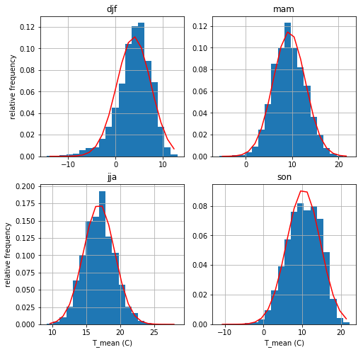
Daily average temperature

The next cell shows histograms temperature for each of the seasons. We use scipy.stats.norm.fit to find the mean and standard deviation (called the loc and scale here) of the data and then shows that fitted distribution as a red line. Specifically, for temperatures x the red line is a plot of:

\begin{align*} f(y) &= \frac{\exp(-y^2/2)}{\sqrt{2\pi}} \\ y &= (x - loc) / scale \end{align*}

The four plots show that a normal distribution give as pretty good representation of each of the seasons.

Missing values again

How many of our temperature measurements are missing? Here’s the count for the whole dataframe

missing_temps=np.sum(np.isnan(yvr_df['T_mean (C)'].values))
missing_precip=np.sum(np.isnan(yvr_df['Total Precip (mm)'].values))
print(f"We are missing {missing_temps} temps and {missing_precip} precips out of {len(yvr_df)} records")

We are missing 24 temps and 25 precips out of 29632 records

So not a showstopper, but still unprofessional/incorrect to set these to 0. Instead we’ll remove them with the dropna method below

key_list = ["djf", "mam", "jja", "son"]
df_list = [season_dict[key] for key in key_list]
#
# set up a 2 row, 2 column grid of figures, and
# turn the ax_array 2-d array into a list
#
fig, ax_array = plt.subplots(2, 2, figsize=(8, 8))
ax_list = ax_array.flatten()
#
# here is the variable we want to histogram
#
var = "T_mean (C)"
#
# store the fit parameters in a dictionary
# called temp_params for future reference
#
temp_params = dict()
#
#  loop over the four seasons in key_list
#  getting the figure axis and the dataframe
#  for that season.
#
for index, key in enumerate(key_list):
    the_ax = ax_list[index]
    the_df = df_list[index]
    the_temps=the_df[var]
    before_drop=len(the_temps)
    the_temps = the_df[var].dropna()
    after_drop=len(the_temps)
    print(f"{before_drop-after_drop} nan values dropped")
    #
    # find the mean and standard deviation to
    # set the pdf mu, sigma parameters
    #
    mu, sigma = st.norm.fit(the_temps)
    #
    # save the parameter pair for that season
    #
    temp_params[key] = (mu, sigma)
    #
    # get the histogram values, the bin edges and the plotting
    # bars (patches) for the histogram, specifying 20 bins
    # note that we can specify the histogram variable by it's dataframe
    # column name when we pass the dataframe to matplotlib via
    # the data keyword
    #
    vals, bins, patches = the_ax.hist(var, bins=20, data=the_df, density=True)
    #
    # turn the bin edges into bin centers by averaging the right + left
    # edge of every bin
    #
    bin_centers = (bins[1:] + bins[0:-1]) / 2.0
    #
    # plot the pdf function on top of the histogram as a red line
    #
    the_ax.plot(bin_centers, st.norm.pdf(bin_centers, mu, sigma), "r-")
    the_ax.grid(True)
    the_ax.set(title=key)
    #
    # label the xaxis for the bottom two plots (2 and 3)
    # and the yaxis for the left plots (0 and 2)
    #
    if index > 1:
        the_ax.set(xlabel=var)
    if index in [0,2]:
        the_ax.set(ylabel='relative frequency')

6 nan values dropped
8 nan values dropped
5 nan values dropped
5 nan values dropped

/Users/phil/mini37/envs/e213/lib/python3.6/site-packages/numpy/lib/histograms.py:824: RuntimeWarning: invalid value encountered in greater_equal
  keep = (tmp_a >= first_edge)
/Users/phil/mini37/envs/e213/lib/python3.6/site-packages/numpy/lib/histograms.py:825: RuntimeWarning: invalid value encountered in less_equal
  keep &= (tmp_a <= last_edge)

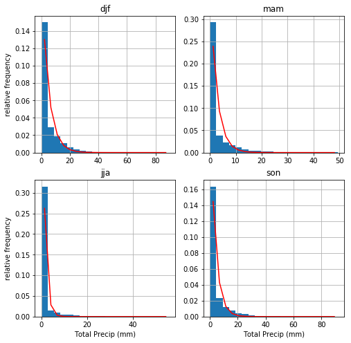
Daily average total precipitation

Precipitation data is a different story. Because negative precipitation is impossible, there is no way a normal distribution is going to work to represent the variablity. Instead we use scipy.stats.expon.fit to fit an exponential distribution.

\begin{align*} f(y) &= \exp(-y)\\ y &= (x - loc) / scale \end{align*}

where loc is the minimum of the data and scale is the distance between the minimum and the mean.

The fits are not quite as good – but do capture the one-sided nature of the variability. No comments on this one, but it’s a copy and paste of the temperature grid plot above.

fig, ax_array = plt.subplots(2, 2, figsize=(8, 8))
ax_list = ax_array.flatten()
var = "Total Precip (mm)"
precip_params = dict()
for index, key in enumerate(key_list):
    the_ax = ax_list[index]
    the_df = df_list[index]
    the_precip = the_df[var]
    before_drop=len(the_precip)
    the_precip = the_df[var].dropna()
    after_drop=len(the_precip)
    print(f"{before_drop-after_drop} nan values dropped")
    loc, scale = st.expon.fit(the_precip)
    precip_params[key] = (loc, scale)
    vals, bins, patches = the_ax.hist(var, bins=20, data=the_df, density=True)
    bin_centers = (bins[1:] + bins[0:-1]) / 2.0
    the_ax.plot(bin_centers, st.expon.pdf(bin_centers, loc, scale), "r-")
    the_ax.grid(True)
    the_ax.set(title=key)
    #
    # label the xaxis for the bottom two plots (2 and 3)
    # and the yaxis for the left plots (0 and 2)
    #
    if index > 1:
        the_ax.set(xlabel=var)
    if index in [0,2]:
        the_ax.set(ylabel='relative frequency')

7 nan values dropped
5 nan values dropped
10 nan values dropped
3 nan values dropped

Saving the fit parameters

We have two new dictionaries: temp_params and precip_params that we should save for the future.

data_dict = dict()
data_dict[
    "metadata"
] = """
          loc,scale tuples for daily average temperature (deg C)
          and precipitation (mm) produced by 11-pandas4 for YVR
          """
data_dict["temp"] = temp_params
data_dict["precip"] = precip_params
fit_file = context.processed_dir / "fit_metadata.json"
with open(fit_file, "w") as f:
    json.dump(data_dict, f, indent=4)

print(f"wrote the fit coefficients to {fit_file}")

wrote the fit coefficients to /Users/phil/repos/eosc213_students/notebooks/pandas/data/processed/fit_metadata.json

#
# here's what the file looks like:
#

with open(fit_file,'r') as f:
    print(f.read())

{
    "metadata": "\n          loc,scale tuples for daily average temperature (deg C)\n          and precipitation (mm) produced by 11-pandas4 for YVR\n          ",
    "temp": {
        "djf": [
            3.8457018498367788,
            3.5951553549810953
        ],
        "mam": [
            9.366519174041297,
            3.4672545858069648
        ],
        "jja": [
            16.897835148581414,
            2.2841620229501727
        ],
        "son": [
            10.315880994430106,
            4.365765620923032
        ]
    },
    "precip": {
        "djf": [
            0.0,
            4.847911848728065
        ],
        "mam": [
            0.0,
            2.6111245141401955
        ],
        "jja": [
            0.0,
            1.2540769644779333
        ],
        "son": [
            0.0,
            3.7721988319978266
        ]
    }
}

Grouping by decade

The two functions below take a season dataframe and create a new column with the decade that each day belongs to. For example if a measurement in taken in 1941, then its decade is 194. We can use that see whether the temperature at the airport has been increasing since the 1930’s and whether that increase depends on season

def find_decade(row):
    """
    given a row from an Environment Canada dataframe
    return the first 3 digits of the year as an integer

    i.e. turn "2010" into the number 201
    """
    year_string=f"{row['Year']:4d}"
    return int(year_string[:3])


def decadal_groups(season_df):
    """
    given a season dataframe produced by groupby('season'), add
    a column called 'decade' with the 3 digit decade
    and return a groupby dictionary of decade dataframes for that
    season with the decade as key
    """
    #
    # add the decade column to the dataframe using apply
    #
    decade=season_df.apply(find_decade,axis=1)
    season_df['decade']=decade
    #
    # do the groupby and turn into a dictionary
    #
    decade_groups=season_df.groupby('decade')
    decade_dict={key:value for key,value in decade_groups}
    return decade_dict

Finding the median temperature

Once we have the dictionary that has the decade as key and the dataframe for that decade as value, we can find the median value of the daily average temperature for each decade using the median_temps function below.

def median_temps(decade_dict):
    """
    given a decade_dict produced by the decadal_temp function
    return a 2-column numpy array.  The first column should be the
    integer decade (193,194,etc.) and the second column should be
    the median temperature for that decade
    """
    values=list()
    for the_decade,the_df in decade_dict.items():
        T_median=the_df['T_mean (C)'].median()
        values.append((the_decade,T_median))
    result=np.array(values)
    return result

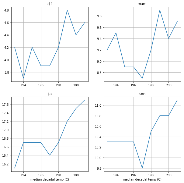
Assignment

Using the functions above, calculate the median temperature for each decade and save your (decade, temperature) lists into a dictionary with a key for each season. Use that dictionary to make a 2 x 2 plot of temperature vs. decade for each of the four seasons, using the 4 box plotting code above. (My solution is 14 lines long)

### BEGIN SOLUTION
season_temps=dict()
for season_key,season_df in season_dict.items():
    decade_dict=decadal_groups(season_df)
    temp_array=median_temps(decade_dict)
    season_temps[season_key]=temp_array

fig, ax_array = plt.subplots(2, 2, figsize=(10, 10))
ax_list = ax_array.flatten()
for index,key in enumerate(key_list):
    temps=season_temps[key]
    the_ax=ax_list[index]
    the_ax.plot(temps[:,0],temps[:,1])
    the_ax.grid(True)
    the_ax.set(title=key)
    if index > 1:
        the_ax.set(xlabel='median decadal temp (C)')
### END SOLUTION