Table of Contents
1 Learning objectives
2 Making random numbers
2.1 Create 1000 uniformly distributed random numbers in the inteval [0,1)
2.2 Repeat for a normal distribution with \(\mu\), and \(\sigma\) from 11-pandas4
2.2.1 First read in the \(\mu\), \(\sigma\) values from fit_metadata.json
2.2.2 Now pull the mean and standard deviation for spring
3 lognormal random numbers with \(\mu=1\), \(\log \sigma=0.1\)
4 Correlated random numbers
5 Your turn
Random number generation
Some examples demonstrating how to generate random numbers using https://docs.scipy.org/doc/numpy/reference/routines.random.html
Learning objectives
Demonstrate random number utilities in numpy.random and scipy.stats
Use the paramter estimates generated by the 11-pandas4 notebook to generate seasonal precipitation and temperature data that fits the observed normal (temperature) and exponential (precipitation) data at YVR airport
Making random numbers
For this notebook, import context defines the Path object for notebooks/pandas/data/processed so that we can find the fit_metadata.json file written by 11-pandas4
[1]:
import numpy as np
import numpy.random as rn
import pandas as pd
from matplotlib import colors
from matplotlib import pyplot as plt
import json
import context
in context.py, found /Users/phil/repos/eosc213_students/notebooks/pandas/data/processed
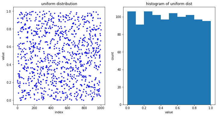
Create 1000 uniformly distributed random numbers in the inteval [0,1)
It’s a good idea to set a seed, so the random numbers will be identical each time you run the notebook
The generator numpy.random.rand generates evenly distributed random numbers between 0 and 1. Below we make 1000 draws and histogram the result.
[2]:
my_seed = 5
rn.seed(my_seed)
uni_dist = rn.rand(1000)
[3]:
fig, (ax1, ax2) = plt.subplots(1, 2, figsize=(12, 6))
ax1.plot(uni_dist, "b.")
ax1.set(title="uniform distribution", ylabel="value", xlabel="index")
ax2.hist(uni_dist)
ax2.set(title="histogram of uniform dist", ylabel="count", xlabel="value");
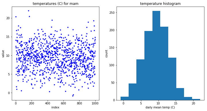
Repeat for a normal distribution with \(\mu\), and \(\sigma\) from 11-pandas4
First read in the \(\mu\), \(\sigma\) values from fit_metadata.json
[4]:
json_file = context.weather_processed_dir / 'fit_metadata.json'
with open(json_file, 'r') as f:
    fit_dict=json.load(f)
fit_dict
[4]:
{'metadata': '\n          loc,scale tuples for daily average temperature (deg C)\n          and precipitation (mm) produced by 11-pandas4 for YVR\n          ',
 'temp': {'djf': [3.84256591465072, 3.595365405560527],
  'mam': [9.356482721671577, 3.4789191637037504],
  'jja': [16.88648212846009, 2.324995343255562],
  'son': [10.308878631550368, 4.372545963729551]},
 'precip': {'djf': [0.0, 4.8432998097309055],
  'mam': [0.0, 2.6093758371283147],
  'jja': [0.0, 1.2523918301531844],
  'son': [0.0, 3.770662503393972]}}
Now pull the mean and standard deviation for spring
[5]:
mu, sigma = fit_dict['temp']['mam']
[6]:
normal_dist = rn.normal(mu, sigma, (1000,))
fig, (ax1, ax2) = plt.subplots(1, 2, figsize=(12, 6))
ax1.plot(normal_dist, "b.")
ax1.set(title="temperatures (C) for mam", ylabel="value", xlabel="index")
ax2.hist(normal_dist)
ax2.set(title="temperature histogram", ylabel="count", xlabel="daily mean temp (C)");
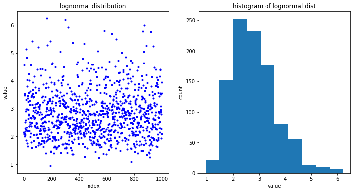
lognormal random numbers with \(\mu=1\), \(\log \sigma=0.1\)
Note that there are dozens of distributions defined by numpy.random
Here is an example for lognormal statistics
[7]:
log_normal_dist = rn.lognormal(1, 0.3, (1000,))
fig, (ax1, ax2) = plt.subplots(1, 2, figsize=(12, 6))
ax1.plot(log_normal_dist, "b.")
ax1.set(title="lognormal distribution", ylabel="value", xlabel="index")
ax2.hist(log_normal_dist)
ax2.set(title="histogram of lognormal dist", ylabel="count", xlabel="value");
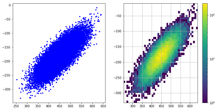
Correlated random numbers
[8]:
def makeRandom(
    meanx=None, stdx=None, meany=None, stdy=None, rho=None, numpoints=100000
):

    """
    return a tuple with two vectors (xvec,yvec) giving the
    coordinates of numpoints chosen from a two dimensional
    Gaussian distribution

    Parameters
    ----------

    meanx: float -- mean in x direction
    stdx:  float -- standard deviation in x direction
    meany: float -- mean in y direction
    stdy:  float -- standar deviation in y direction
    rho:   float -- correlation coefficient
    numpoints:  length of returned xvec and yvec


    Returns
    -------

    (xvec, yvec): tuple of ndarray vectors containing
                  correlated random variables,
                  each vector of length numpoints

    Example
    -------

    invalues={'meanx':450.,
              'stdx':50,
              'meany':-180,
              'stdy':40,
              'rho':0.8}

    chanx,chany=makeRandom(**invalues)


    """
    sigma = np.array([stdx ** 2.0, rho * stdx * stdy, rho * stdx * stdy, stdy ** 2.0])
    sigma.shape = [2, 2]
    meanvec = [meanx, meany]
    outRandom = rn.multivariate_normal(meanvec, sigma, [numpoints])
    chan1 = outRandom[:, 0]
    chan2 = outRandom[:, 1]
    return (chan1, chan2)
[9]:
invalues = {
    "meanx": 450.0,
    "stdx": 50,
    "meany": -180,
    "stdy": 40,
    "rho": 0.8,
    "numpoints": 25000,
}

chanx, chany = makeRandom(**invalues)
[10]:
# https://matplotlib.org/gallery/statistics/hist.html
fig, (ax1, ax2) = plt.subplots(1, 2, figsize=(12, 6))
ax1.plot(chanx, chany, "b.")
h, x, y, im = ax2.hist2d(chanx, chany, bins=(50, 50), norm=colors.LogNorm())
fig.colorbar(im)
ax2.grid(True)
Your turn
Generate a precipitation dataset for YVR springtime using numpy.random.exponential
We have been assuming that precipitation and temperature are independent random variables. Make a scatterplot and 2D histogram of one of the YVR seasonal precipitation, temperature dataframes. Do you see any correlation? What does numpy.correlate say?
[ ]: