Table of Contents
1 Solving Ordinary Differential Equations
1.1 Objectives
1.2 Introduction
1.3 Euler’s methods
1.3.1 From the mass balance to the ODE
1.3.2 Analytical Solution
1.4 Integral form of the ODE
1.4.1 Euler’s approach
1.4.2 Examples of application
1.4.3 Runge Kutta methods
Solving Ordinary Differential Equations
Objectives
In this lecture, we will review the main computational techniques to solve a first order differential problem (initial value problem) of the type:
\begin{equation} \left\lbrace \begin{array}{lll} \displaystyle{\frac{dy}{dt}} & = & f(y,t) \\ y(t_0) & = & y_0 \end{array} \right. \end{equation}
Specifically you will be able to:
link the ODE to a physical problem
develop different computational methods to solve the initial value problem
understand the concept of stability and accuracy of a computation methods
describe Euler forward and backward approaches
Introduction
Ordinary differential equations (ODEs) arise in many physical situations. For example, there is the second-order Newton’s Second Law of Mechanics \(F=ma\) .
In general, higher-order equations, such as Newton’s force equation, can be rewritten as a system of first-order equations. So the generic problem in ODEs is a set of N coupled first-order differential equations of the form defined above.
where \({\bf y}\) is a vector of variables. As an example, the Newton’s law of motion could be written as
Which is a second order differential equation. But nothing can prevent us from describing the same problem through two first-order coupled ODEs:
\begin{equation} \left\lbrace \begin{array}{lll} \displaystyle{\frac{dx}{dt}} & = & v_x(x,t) \\ \displaystyle{m\frac{dv_x}{dt}} & = & F(x,t) \\ \end{array} \right. \end{equation}
That means that we can limit our next discussions to the first order problems.
Euler’s methods
In engineering, conceptual models will describe how a certain quantity (mass, energy, position, …) will evolve: it is about identifying which processes will affect that quantity, and translate them into a mathematical form.
From the mass balance to the ODE
Source and sink terms
For the sulfates TMF problem, we had identified 4 contributions to the sulfate concentration.
\(M_{\text{pit}}\) is the mass of sulfates added over \(\Delta t\) from the mill (mg).
\(M_{\text{mill}}\) is the mass of sulfates added over \(\Delta t\) from the pit (mg).
\(M_{\text{pore}}\) is the mass of sulfates added over \(\Delta t\) from that exchange term with the tailings porewater (mg)
\(M_{\text{discharge}}\) is the mass of sulfates removed over \(\Delta t\) from the discharge flux (mg)
Therefore, if the mass of sulfates at a certain time \(t_0\) is \(m(t_0) = m_0\), the mass of sulfates at \(t_0 + \Delta t\) is: \begin{equation} m(t_0 + \Delta t) = m(t_0) + M_{\text{pit}} + M_{\text{mill}} + M_{\text{pore}} - M_{\text{dis}} \end{equation}
And we have identified these terms:
\begin{equation} \left\lbrace \begin{array}{lll} M_{\text{pit}} & = & Q_{\text{pit}}c_{\text{pit}} \Delta t\\ M_{\text{mill}} & = & Q_{\text{mill}}c_{\text{mill}} \Delta t\\ M_{\text{pore}} & = & kA_{\text{bottom}}(c_{\text{pore}} - c_{\text{TMF}}) \Delta t\\ M_{\text{discharge}} & = & Q_{\text{dis}}c_{\text{TMF}} \Delta t\\ \end{array} \right. \end{equation}
So we can rewrite the previous equation as:
\begin{equation} \begin{array}{llll} & m(t_0 + \Delta t) & = & m(t_0) + M_{\text{pit}} + M_{\text{mill}} + M_{\text{pore}} - M_{\text{dis}} \\ \Longleftrightarrow & m(t_0 + \Delta t) & = & m(t_0) + \left(Q_{\text{pit}} c_{\text{pit}} + Q_{\text{mill}} c_{\text{mill}} + A_{\text{bottom}} k \left( c_{\text{pore}} - c_{\text{TMF}} \right) -Q_{\text{dis}} c_{\text{TMF}}\right) \Delta t \\ \Longleftrightarrow & \frac{m(t_0 + \Delta t)-m(t_0)}{\Delta t} & = & Q_{\text{pit}} c_{\text{pit}} + Q_{\text{mill}} c_{\text{mill}} + A_{\text{bottom}} k \left( c_{\text{pore}} - c_{\text{TMF}} \right) -Q_{\text{dis}} c_{\text{TMF}} \\ \end{array} \end{equation}
The link between concentration and mass of sulfates is the volume of water \begin{equation} c_{\text{TMF}}(t) = \frac{m(t)}{V(t)} \end{equation}
But, since the volume of water is constant (\(V_0\)), we have: \begin{equation} c_{\text{TMF}}(t) = \frac{m(t)}{V_0} \end{equation}
Therefore, if we divide the latter equation by \(V_0\), we have: \begin{equation} \frac{c_{\text{TMF}}(t + \Delta t)-c_{\text{TMF}}(t)}{\Delta t} = \frac{Q_{\text{pit}} c_{\text{pit}} + Q_{\text{mill}} c_{\text{mill}} + A_{\text{bottom}} k \left( c_{\text{pore}} - c_{\text{TMF}} \right) -Q_{\text{dis}} c_{\text{TMF}}}{V_0} \end{equation}
So, after each time step, we can compute the evolution of \(c_{\text{TMF}}\). How should we choose the timestep?
It is irrelevant
It should be as small as possible
The bigger the faster
The choice of the timestep matters. Look at the previous equation:
\begin{equation} \frac{\color{blue}{c_{\text{TMF}}}(t + \Delta t)-c_{\text{TMF}}(t)}{\Delta t} = \frac{Q_{\text{pit}} c_{\text{pit}} + Q_{\text{mill}} c_{\text{mill}} + A_{\text{bottom}} k \left( c_{\text{pore}} - {\color{red}{c_{\text{TMF}}}} \right) -Q_{\text{dis}} \color{red}{c_{\text{TMF}}}}{V_0} \end{equation}
To compute the solution \(c_{\text{TMF}}(t+ \Delta t)\), we use the value of \(c_{\text{TMF}}\). But, at what time? Intrinsically, at every time between \(t\) and $ t + \Delta `t$, the value of :math:`c_{\text{TMF}} changes.
So the timestep should be small!
ODE
Going to the limit \(\Delta t \rightarrow 0\) (i.e. \(\Delta t= dt\), \(c(t+\Delta t)-c(t)= dc\)), the equation becomes: \begin{equation} \frac{dc_{\text{TMF}}}{dt} = \frac{Q_{\text{pit}} c_{\text{pit}} + Q_{\text{mill}} c_{\text{mill}} + A_{\text{bottom}} k \left( c_{\text{pore}} - c_{\text{TMF}} \right) -Q_{\text{dis}} c_{\text{TMF}}}{V_0} \end{equation} which is a 1\(^{st}\) order linear ODE.
Asymptotic behavior
Let us build a bit of physical sense is often a good idea. One should realize that this problem is bound to have a steady solution (a solution which does not evolve in time). This is not always true. But, in this case, at some point, the concentration in the TMF will be so that the sink term will exactly compensate the source terms.
This happens when the derivative is zero!
\begin{equation} \begin{array}{lll} & \frac{dc_{\text{TMF}}}{dt} & = & 0 \\ \Longleftrightarrow & 0 & = & \frac{Q_{\text{pit}} c_{\text{pit}} + Q_{\text{mill}} c_{\text{mill}} + A_{\text{bottom}} k \left( c_{\text{pore}} - c_{\text{TMF}} \right) -Q_{\text{dis}} c_{\text{TMF}}}{V_0} \\ \Longleftrightarrow & c_{\text{TMF}} & = & \frac{Q_{\text{pit}} c_{\text{pit}} + Q_{\text{mill}} c_{\text{mill}} + kA c_{\text{pore}} }{Q_{\text{dis}}+kA} \equiv c_\infty \end{array} \end{equation}
The asymptotic/final concentration (the steady-state concentration) \(c_\infty\) corresponds to the final solution.
Can you try to guess which values \(c_\infty\) could be?
Let us analyse this by investigating limit cases:
Very fast production from the porewater: \(k \rightarrow \infty\) :nbsphinx-math:`begin{equation} begin{array}{lll} c_infty & = & frac{Q_{text{pit}} c_{text{pit}} + Q_{text{mill}} c_{text{mill}} + kA c_{text{pore}} }{Q_{text{dis}}+kA} \
- & = & frac{color{blue}{Q_{text{pit}} c_{text{pit}}} + color{blue}{Q_{text{mill}} c_{text{mill}}} + kA c_{text{pore}} }{color{blue}{Q_{text{dis}}}+kA} \
& approx & frac{kA c_{text{pore}} }{kA} \
& approx & c_{text{pore}} = 2000 text{ mg/L}
end{array} end{equation}`
Very slow production from the porewater: \(k \rightarrow 0\) :nbsphinx-math:`begin{equation} begin{array}{lll} c_infty & = & frac{Q_{text{pit}} c_{text{pit}} + Q_{text{mill}} c_{text{mill}} + kA c_{text{pore}} }{Q_{text{dis}}+kA} \
- & = & frac{Q_{text{pit}} c_{text{pit}} + Q_{text{mill}} c_{text{mill}} + color{blue}{kA c_{text{pore}}} }{Q_{text{dis}}+color{blue}{kA}} \
& approx & frac{Q_{text{pit}} c_{text{pit}} + Q_{text{mill}} c_{text{mill}}}{Q_{text{dis}}} \
& approx & 256.82 text{ mg/L}
end{array} end{equation}`
Therefore, the asymptotic concentration should never be outside these two bounds!
Analytical Solution
The ODE can be rewritten in the following way:
\begin{equation} \frac{dc_{\text{TMF}}}{dt} + \lambda c_{\text{TMF}} = Q \end{equation} with \begin{equation} \left\lbrace \begin{array}{lll} Q & = & \frac{Q_{\text{pit}}c_{\text{pit}} + Q_{\text{mill}}c_{\text{mill}}+ kAc_{\text{pore}}}{V_0} \\ \lambda & = & \frac{Q_{\text{dis}}+kA}{V_0} \end{array} \right. \end{equation}
You can notice that \begin{equation} c_\infty = \frac{Q}{\lambda} \end{equation}
The associated homogeneous problem is \begin{equation} \begin{array}{ll} & \frac{dc_{\text{TMF}}}{dt} + \lambda c_{\text{TMF}} = 0 \\ \Longleftrightarrow & \frac{dc_{\text{TMF}}}{dt} = -\lambda c_{\text{TMF}} \\ \end{array} \end{equation}
In other words, we are trying to find a function which is proportional to its opposite.
Any idea?
The solution of the homogeneous problem \(c_H\) is \begin{equation} c_H(t) = A \mathrm{exp}(-\lambda t) \end{equation}
The solution to the particular problem should arise from our physical sense. We know that the solution should reach a steady-state, so a particular solution is a constant solution \(c_p(t) = c\).
By injecting that solution into the differential problem, we find:
\begin{equation} c_p(t) = c = \frac{Q}{\lambda} = c_\infty \end{equation}
which corresponds to our physical sense!
So that the general solution to the ODE is: \begin{equation} c_{\text{TMF}}(t) = c_\infty + A \mathrm{exp}(-\lambda t) \end{equation}
The last thing to do is to find the value of A so that the initial concentration meets our given problem. Usually, initial means at \(t=0\), but you can take any other value of time \(t_0\), as long as you are consistent with that value later.
We know that: \begin{equation} c(0) = c_0 (=93) \Longleftrightarrow c_\infty + A = c_0 \Longleftrightarrow A = c_0 - c_\infty \end{equation}
So the exact solution of the problem: \begin{equation} c_{\text{TMF}}(t) = c_\infty + \left( c_0 - c_\infty \right) \mathrm{exp}(-\lambda t) \end{equation}
So, what would happen if you arbitrarly chose \(t_0\) to be something else than 0? For example, if you want \(t_0\) to be the age of the universe, then, \(c_{\text{TMF}}\) has to match 93 mg/L after 4.343 \(\times\) 10\(^{17}\)seconds (13.772 billions of years!). That would give you a value A. As long as you stick to that value of A and to that initial \(t_0\), the following solution will be the same. But computationnally, the difference between 13 billions of years and 13 billions + 1 year might be lost in rounding erros… So it’s probably not the greatest idea!
The fact that we know the exact solution to a problem allows us to assess the accuracy of a computational approach. Let us take a look at the solution!
[13]:
# Parameters definition
import numpy as np
from matplotlib import pyplot as plt

c_pit = 50
c_pore = 2000
c_mill = 700
Q_pit = 30
Q_mill = 14
Q_dis = 44
V0 = 8.1e9
c0 = 93  # initial concentration
k = 2.5e-5
Area = 3e5
#
# Eqn 13
#
c_inf = (Q_pit * c_pit + Q_mill * c_mill + Area * k * c_pore) / (Q_dis + Area * k)
A = c0 - c_inf
lam = (Area * k + Q_dis) / V0  # units are here in s^{-1}
#
# Eqn 15
#
Q = (Q_pit * c_pit + Q_mill * c_mill + Area * k * c_pore) / V0
print(lam)
print(Q)
6.358024691358025e-09
3.2469135802469134e-06
[14]:
# This is the routine to plot the exact solution for the concentration at every day
dt = 1 # day
Tf = 50 # years
n = int(1 + 365 * Tf / dt) # int() is to convert thhe result into an integer
c_real = np.zeros(
n, float
) # represents the concentration of sultates (mg/L) at each time
timeY = np.zeros(n, float) # time in years
c_real[0] = c0
c_asymptotic = c_inf * np.ones(
n, float
) # this is an array of size n, whose values are all c_inf
#
# Eq. 22
#
for i in range(n - 1):
timeY[i + 1] = (i + 1) * dt / 365
c_real[i + 1] = c_inf + (c0 - c_inf) * np.exp(-lam * (i + 1) * dt * 3600 * 24)
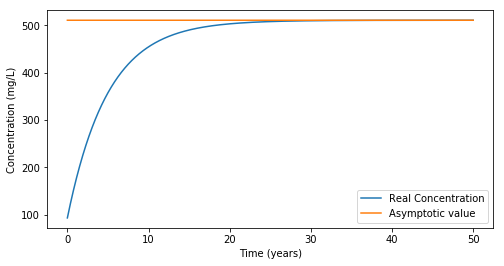
fig, (ax1) = plt.subplots(1, 1, figsize=(8, 4))
ax1.plot(timeY, c_real, label="Real Concentration")
ax1.plot(timeY, c_asymptotic, label="Asymptotic value")
ax1.set(xlabel="Time (years)", ylabel="Concentration (mg/L)")
ax1.legend()
print(
f"Asymptotic concentration is: {c_inf} mg/L,\n"
f"exact concentration after {Tf} years is {c_real[n-1]}"
)
Asymptotic concentration is: 510.6796116504854 mg/L,
exact concentration after 50 years is 510.6611233781182
Integral form of the ODE
The general 1\(^{st}\) order ODE is written in the form
\begin{equation} \frac{dy}{dt} = f(y,t) \Longleftrightarrow dy = f(y,t)dt \end{equation}
If the ODE is not separable (meaning the function \(f(y,t)\) cannot be split into function \(f(y,t)=Y(y)T(t)\), we cannot apply the variable separation method.
We can therefore write: \begin{equation} \int dy = \int_{t_0}^{t_0+\Delta t} f(y,t)dt \end{equation}
which leads to
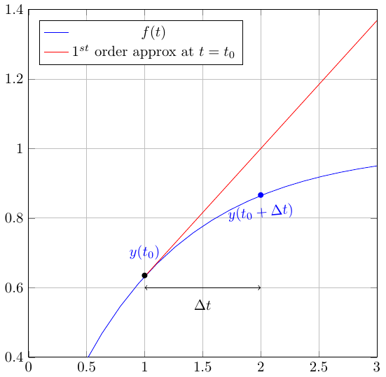
\begin{equation} y(t_0+\Delta t) = y(t_0) + \int_{t_0}^{t_0+\Delta t} f(y,t)dt \end{equation}
[4]:
from IPython.display import Image

Image(filename="figures/figinit.png")
[4]:
Euler’s approach
The two Euler’s methods are a way to compute this integral term. They both work on the approximation that the function \(f(y,t)\) is constant over the timestep [\(t\);\(t+\Delta t\)].
Forward Euler
The forward Euler approach consists in the following approximation:
\begin{equation} f(y,t) \approx f(y_0,t_0) \text{ between [$t_0$;$t_0+\Delta t$]} \end{equation}
[5]:
Image(filename="figures/figExplicitEuler.png")
[5]:
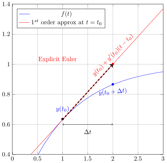
This approximation allows us to write:
\begin{equation} \begin{array}{lll} \int_{t_0}^{t_0 + \Delta t} f(y,t)dt & \approx & f(y_0,t_0) \int_{t_0}^{t_0 + \Delta t} dt \\ & \approx & f(y,t_0) \Delta t \end{array} \end{equation}
The forward Euler method takes the solution at time \(t_n\) and advances it to time \(t_{n+1}\) using the value of the derivative \(f(y_n,t_n)\) at time \(t_n\)
This is also referred to as the explicit approach, as the new value of function \(y\) can be computed immediately (i.e. explicitly) from the previous expression.
Backward Euler
The backward Euler method is very similar in principle but its application leads to very different results (forward approach is almost never used for stability issues, see below). The forward Euler approach consists in the following approximation:
\begin{equation} f(y,t) \approx f(y,t_0+\Delta t) \text{ between [$t_0$;$t_0+\Delta t$]} \end{equation}
[6]:
Image(filename="figures/figImplicitEuler.png")
[6]:
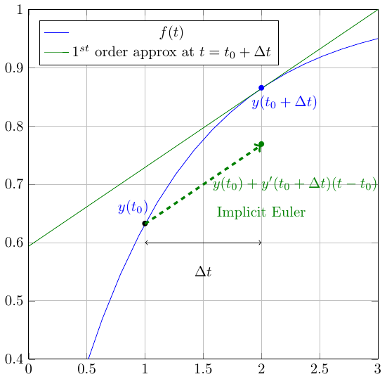
This approximation allows us to write:
\begin{equation} \begin{array}{lll} \int_{t_0}^{t_0 + \Delta t} f(y,t)dt & \approx & f(y,t_0+\Delta t) \int_{t_0}^{t_0 + \Delta t} dt \\ & \approx & f(y,t_0+\Delta t) \Delta t \end{array} \end{equation}
Back in the initial ODE, this yields: \begin{equation} y(t_0+\Delta t) = y(t_0) + f(y,t_0+\Delta t) \Delta t \end{equation}
Which is an equation which has to be solved. Depending on the form of the function \(f\), this might be a nonlinear equation to solve. We will see later examples of methods to solve these problems (Newton method, for example).
Examples of application
We have shown that the associated ODE to the sulate problem could be written as:
\begin{equation} \frac{dc_{\text{TMF}}}{dt} + \lambda c_{\text{TMF}} = Q \end{equation} with \begin{equation} \left\lbrace \begin{array}{lllll} Q & = & \frac{Q_{\text{pit}}c_{\text{pit}} + Q_{\text{mill}}c_{\text{mill}}+ kAc_{\text{pore}}}{V_0} & \approx & 3.247 \times 10^{-6} mg . L^{-1} . s^{-1} \\ \lambda & = & \frac{Q_{\text{dis}}+kA}{V_0} & \approx & 6.358 \times 10^{-9} s^{-1} \end{array} \right. \end{equation}
The forward Euler’s method yields: \begin{equation} c(t_0 + \Delta t) = c(t_0) + \left( Q - \lambda c(t_0) \right) \Delta t \end{equation}
While the backward Euler’s method yields: \begin{equation} \begin{array}{llll} & c(t_0 + \Delta t) & = & c(t_0) + \Delta t (Q - \lambda c(t_0+\Delta t)) \\ \Longleftrightarrow & c(t_0 + \Delta t) \left( 1 + \lambda \Delta t \right) & = & c(t_0) + Q \Delta t \\ \Longleftrightarrow & c(t_0 + \Delta t) & = & \displaystyle{\frac{c(t_0) + Q \Delta t}{1 + \lambda \Delta t}} \\ \end{array} \end{equation}
So, let us compare these solutions to the analytical solution. We will therefore compute the two Euler approaches at each timestep and assess the error of the solution.
[7]:
# This is the routine to plot the exact solution for the concentration at every day
dt = 1  # day
Tf = 50  # years
n = int(1 + 365 * Tf / dt)  # int() is to convert thhe result into an integer
c_real = np.zeros(
    n, float
)  # represents the concentration of sultates (mg/L) at each time
timeY = np.zeros(n, float)  # time in years
c_real[0] = c0
c_asymptotic = c_inf * np.ones(
    n, float
)  # this is an array of size n full, whose values are all c_inf
Forward_Euler = np.zeros(n, float)
Backward_Euler = np.zeros(n, float)
err_Backward = np.zeros(n, float)
err_Forward = np.zeros(n, float)
Forward_Euler[0] = c0
Backward_Euler[0] = c0


for i in range(n - 1):
    timeY[i + 1] = (i + 1) * dt / 365
    c_real[i + 1] = c_inf + (c0 - c_inf) * np.exp(-lam * (i + 1) * dt * 3600 * 24)
    Forward_Euler[i + 1] = 0 #ADAPT THIS
    Backward_Euler[i + 1] = # ADAPT THIS
    err_Backward[i + 1] = (c_real[i + 1] - Backward_Euler[i + 1]) / c_real[i + 1]
    err_Forward[i + 1] = (Forward_Euler[i + 1] - c_real[i + 1]) / c_real[i + 1]

fig, (ax1, ax2) = plt.subplots(2, 1, figsize=(8, 8))
ax1.plot(timeY, c_real, label="Real Concentration")
ax1.plot(timeY, Forward_Euler, label="Concentration - Forward Euler")
ax1.plot(timeY, Backward_Euler, label="Concentration - Backward Euler")
ax1.set(xlabel="Time (years)", ylabel="Concentration (mg/L)")
ax1.legend()

ax2.plot(timeY, 100 * err_Backward, label="Error - backward Euler")
ax2.plot(timeY, 100 * err_Forward, label="Error - forward Euler")
ax2.set(xlabel="Time (years)", ylabel="Error (%)")
ax2.legend()
[7]:
<matplotlib.legend.Legend at 0x7f1d93db0a90>
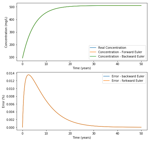
We can see that the two approaches are quite close to each other and to the analytical solution. This means that the approximation is good. When you calculated the sulfates concentration after 1 day, you saw that it had increased from 93 to 93.23 mg/L, hence a relative increase of 0.2%. This yields that the approximation that \(c_{\text{TMF}}\) is constant over a day is pretty good, hence a relatively small error!
So, the bigger the timestep, the less accurate is the approximation. Let us check that! We will set a timestep of 5 years and see the effect on the result and the error.
[15]:
dt = 5 * 365  # day
Tf = 50  # years
n = int(1 + 365 * Tf / dt)  # int() is to convert thhe result into an integer

timeY = np.linspace(0, Tf, n)  # this is a way to create an array of size n,
# which starts at 0, ends at Tf and every elements
# are evenly spaced
c_real = np.zeros(
    n, float
)  # represents the concentration of sultates (mg/L) at each time
# timeY             = np.zeros(n, float) # time in years
c_real[0] = c0
c_asymptotic = c_inf * np.ones(
    n, float
)  # this is an array of size n full, whose values are all c_inf
Forward_Euler = np.zeros(n, float)
Backward_Euler = np.zeros(n, float)
err_Backward = np.zeros(n, float)
err_Forward = np.zeros(n, float)
Forward_Euler[0] = c0
Backward_Euler[0] = c0


for i in range(n - 1):
    # timeY[i+1]          = (i+1)*dt/365
    c_real[i + 1] = c_inf + (c0 - c_inf) * np.exp(-lam * timeY[i + 1] * 365 * 3600 * 24)
    Forward_Euler[i + 1] = 0
    Backward_Euler[i + 1] = 0
    err_Backward[i + 1] = 0
    err_Forward[i + 1] = 0

fig, (ax1, ax2) = plt.subplots(2, 1, figsize=(8, 8))
ax1.plot(timeY, c_real, label="Real Concentration")
ax1.plot(timeY, Forward_Euler, label="Concentration - Forward Euler")
ax1.plot(timeY, Backward_Euler, label="Concentration - Backward Euler")
ax1.set(xlabel="Time (years)", ylabel="Concentration (mg/L)")
ax1.legend()

ax2.plot(timeY, 100 * err_Backward, label="Error - backward Euler")
ax2.plot(timeY, 100 * err_Forward, label="Error - forkward Euler")
ax2.set(xlabel="Time (years)", ylabel="Error (%)")
ax2.legend()
[15]:
<matplotlib.legend.Legend at 0x7f1d93a3cac8>
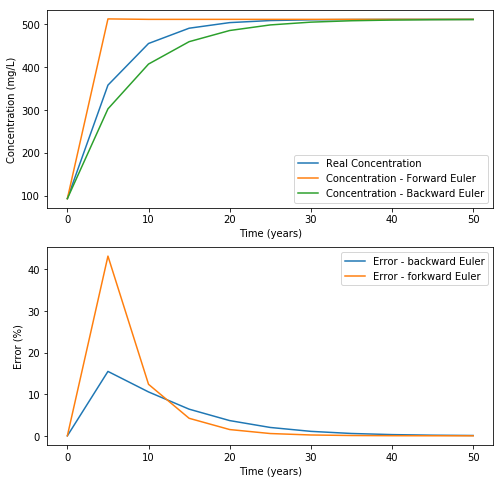
This defines the accuracy of the algorithm. The accuracy decreases when the timestep increases!
Basically, Euler’s method states that here, for the first 5 years, the source term from the tailings porewater is at its maximum, and the discharge is at its minimum for the forward Euler’s approach. We therefore have a very important overestimation of the source and underestimation of the sink, which yields an important overestimation of the error.
Now, do the same with an even bigger timestep (25 years and see what is happening over a longer timescale, like 250 years).
[9]:
### YOUR CODE HERE
[9]:
<matplotlib.legend.Legend at 0x7f1d93c073c8>
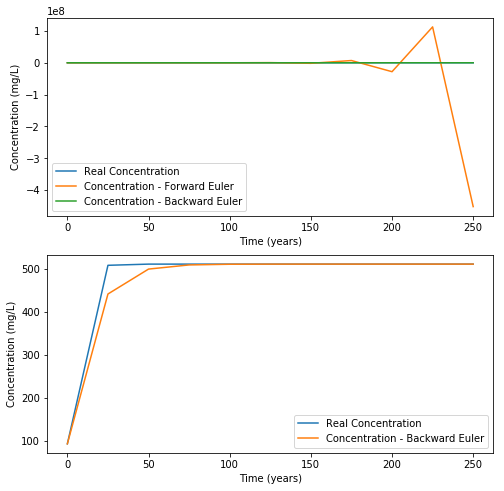
This defines the concept of stability.
We can show that Euler’s backward method is unconditionnally stable (for every timestep), while Euler’s forward (explicit) method has a restrictive timestep condition for stability.
That is one of the reason why Euler’s backward (implicit) method is usually preferred than the Euler’s forward (explicit approach). However, this yields 1. In most case (depending on \(f(y,t)\)), there is an equation to solve (often numerically) to find the value of \(y(t+\Delta t)\) 2. Stability does not mean accuracy
These methods are referred to as 1\(^{st}\) order methods. The order of the method is linked to the Taylor approximation
\begin{equation} y(t+\Delta t) = y(t) + (\Delta t) y^\prime(t) + \frac{1}{2}(\Delta t)^2 y^{\prime\prime}(t) +\cdots \end{equation}
So, as the function f is the derivative of \(y\), the Euler’s approach omits all the term but the 1\(^{st}\) order: it is called a first order method (also we use \(y = y_0 + \Delta t f\)). We compute the evolution of the solution based on the first order approximation of \(y\) (we assume a constant value for its derivative \(f\)).
The truncation error corresponds to the omission of all the higher order terms:
\begin{equation} \text{Truncation error } = \frac{1}{2}(\Delta t)^2 y^{\prime\prime}(t) +\cdots \end{equation}
So, the intrinsic error we make with Euler’s methods is proportional to \((\Delta t)^2\). In words, we say that forward Euler is first order accurate with errors of second order. It is therefore clear that reducing the timestep reduces the errors.
Runge Kutta methods
In a lot of applications, Euler’s implicit method is used. But in some cases, higher order and more accurate methods need to be used. They basically compute the integral
with more accuracy (with a higher-order). These are commonly known as the Runge-Kutta methods (Euler’s methods are a 1st order Runge-Kutta method). The idea of the Runge-Kutta schemes is to take advantage of derivative information at the times between \(t_n\) and \(t_{n+1}\) to increase the order of accuracy.
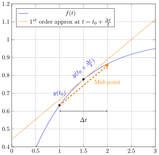
For example, in the midpoint method, the derivative at the initial time is used to approximate the derivative at the midpoint of the interval, \(f(y_n+\frac{1}{2}hf(y_n,t_n), t_n+\frac{1}{2}h)\). The derivative at the midpoint is then used to advance the solution to the next step. The method can be written in two stages \(k_i\),
- :nbsphinx-math:`begin{equation}
- begin{array}{lll}
k_1 & = & Delta t f(y(t),t)\ k_2 & =& Delta t , fleft( y(t)+frac{1}{2}k_1, t+frac{1}{2}Delta t right)\y(t+Delta t) & =& y(t) + k_2
end{array}
end{equation}`
The midpoint method is known as a 2-stage Runge-Kutta formula.
[10]:
Image(filename="figures/figMidpoint.png")
[10]:
In general, an explicit 2-stage Runge-Kutta method can be written as,
- :nbsphinx-math:`begin{equation}
- begin{array}{l}
k_1 = h f(y(t),t)\ k_2 = Delta t f left( y(t)+b_{21}k_1, t+a_2h right) \ y(t+Delta t) = y(t) + c_1k_1 +c_2k_2
end{array}
end{equation}`
It is said explicit because the new solution only depends on the previous solution. The different coefficient can be determined by comparison with the 2\(^{nd}\) order Taylor approximation.
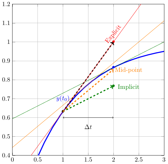
[12]:
Image(filename="figures/fig-Summary.png")
[12]: