Table of Contents
1 Introduction to computational methods
1.1 Data file
1.2 Algorithm
1.3 Python code
1.4 Python modules/libraries
1.5 convert flow to a numpy array
Introduction to computational methods
This notebook introduces a python program to integrate daily average flow into and out of the tailings management facility (TMF), and the volume of water in the TMF through time.
Data file
This notebook assumes that a comma-separated variable (csv) file named data/july2016-tmf-flow.csv exists in the data folder in the current working directory. The file contains three columns with headers:
date outflow inflow
The first 4 lines of the file are:
date,outflow,inflow 2016-07-01,0.0703,0.1181 2016-07-02,0.066,0.1121 2016-07-03,0.0621,0.1079
The data in the csv file is in the following format
date is in yyyy-mm-dd
outflow is the daily average outflow in \(m^3/s\)
inflow is the daily average inflow in \(m^3/s\)
Algorithm
The volume of water in the TMF on day \(t\) of the computation is \(V(t)\), the daily average outflow is \(Q_{out}\) and the daily average inflow is \(Q_{out}\)
The basic computational algorithm is:
Read in the date, \(Q_{out}\) and \(Q_{out}\) data from the file
july2016-tmf-flow.csv.Compute the change in volume over the day \(\Delta V = (Q_{in} - Q_{out})\Delta t\)
Update the volume of the TMF: \(V(t+\Delta t) = V(t) + \Delta V\)
Loop through all dates in the file until complete.
Python code
We’ll introduce python concepts as we go in the course, so we don’t expect you to fully understand this code yet. We’ll therefore only provide a cursory explanation here.
Python modules/libraries
It is good practice to import libaries at the beginning of a program. Libaries are collections of python code.
[1]:
import matplotlib.dates as mdates
import matplotlib.pyplot as plt
import numpy as np
import pandas as pd
The import command tells python to import the library. The as specifies a user - chosen nickname for library to be used in this program. So for this program, the numpy library will also be known as np.
We are importing four libraries or library sections:
numpy is a library with numerical - related codes. We’ll use it alot in the course.
pandas is a libary with codes to manipulate tabular data, that is data organized in rows and columns.
matplotlib is a vast library for plotting. We don’t need the whole library, but only two subsections.
matplotlib.pyplot, nicknamed plt is a subsection containing so-called handle graphics. We’ll use it alot.
matplotlib.dates, which we nickname mdates is a specialty subsection containing code for manipulating date formats.
[2]:
# use pandas to read in csv data
data_file = "data/july2016-tmf-flow.csv"
df_flow = pd.read_csv(data_file)
df_flow.head()
[2]:
| date | outflow | inflow | |
|---|---|---|---|
| 0 | 2016-07-01 | 0.0703 | 0.1181 |
| 1 | 2016-07-02 | 0.0660 | 0.1121 |
| 2 | 2016-07-03 | 0.0621 | 0.1079 |
| 3 | 2016-07-04 | 0.0599 | 0.1115 |
| 4 | 2016-07-05 | 0.0574 | 0.1108 |
The pd.read_csv command from the pandas library reads all the rows and columns from the file july2016-tmf-flow.csv.
We could have also written the command as pandas.read.csv, but we used our nickname pd to save some typing.
Here we see the power of the pandas library. This command contains code to open the file, read in each line of data from the csv file,and then stores that data in a dataframe that we named flow. You can think of a dataframe as rows and columns of data. In our case, the data in the dataframe is dates, outflows and inflows.
convert flow to a numpy array
[3]:
flow = df_flow.values

# find number of days of data (number of rows in array)

n = flow.shape[0]
print(f"Number of days in file: {n}")
flow[:4, :]
Number of days in file: 31
[3]:
array([['2016-07-01', 0.0703, 0.1181],
       ['2016-07-02', 0.066, 0.1121],
       ['2016-07-03', 0.0621, 0.1079],
       ['2016-07-04', 0.0599, 0.1115]], dtype=object)
This line of code uses the .shape method, which returns the dimension (number of rows and columns) in the dataframe flow. .shape[0] is the number of rows, or in our case, the number of days of outflow and inflow data in the dataframe, which we assign to the variable n.
[4]:
# allocate np arrays for time and volume for calculations -
# doing this in advance makes python run faster

v = np.zeros(n, float)
The function zeros from the numpy library creates an array of zeros. Python runs faster if the arrays used for computation are defined in advance, versus on the fly. Here we create an array v of n zeros of type float. Each element in v will store the volume of water in the TMF on a specific day.
[5]:
# print  the columns in the dataframe
print(f"Columns in csv file: {df_flow.columns}")

# convert column called date to pandas date format
# and store in column called yearmonthday

df_flow["yearmonthday"] = pd.to_datetime(df_flow["date"])

# see the data in the column yearmonthday
print(f"type of the timestap object: {type(df_flow['yearmonthday'][0])}")
Columns in csv file: Index(['date', 'outflow', 'inflow'], dtype='object')
type of the timestap object: <class 'pandas._libs.tslibs.timestamps.Timestamp'>
We first print the names of the columns in the dataframe that were read in from the csv file. We do this using the .columns method on the flow dataframe; that is flow.columns returns the indices of the columns in the dataframe.
The command flow["yearmonthday"] = pd.to_datetime(flow["date"] uses the pandas method .to_datetime to convert the data in the column indexed with date in the dataframe flow to a date format that pandas understands, and then stores those panda dates in the dataframe flow in a new column with index yearmonthday.
We then print out the type of the data in the column yearmonthday to prove that it is now a date.
[6]:
# set volume in TMF at time zero to 8.1 x 10^6 m^3

v[0] = 8.1e6

"""
loop through and compute volume through time
since flow is in m^3/s, and flows are daily average flows, must convert
to m^3 in a day by multiplying by 86400 s/d
"""
seconds_per_day = 86400.0
inflow = flow[:, 1]
outflow = flow[:, 2]
for i in range(n - 1):
    v[i + 1] = v[i] + (inflow[i] - outflow[i]) * seconds_per_day

df_flow["volume"] = v
This is the guts of the computation. We first set the volume in the TMF at time zero to \(8.1\times 10^6 m^3\).
Then we loop through the days in the dataframe and compute the change in volume over each day as described above: \(V(t+\Delta t) = V(t) + (Q_{in} - Q_{out})\Delta t\), where \(\Delta t\) is \(86400\) seconds (one day).
In python we use a for loop. The command for i in range(n - 1): sets i to 0, then enters the loop and when finished the loop, sets i to 1, enters the loop,…, n-1. On the last time through the loop, i=n-1 so that when we computev[i+1] for the last time, we are computing v[n].
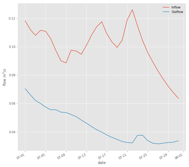
The rest of the code is used to generate the plot of outflow and inflow over time in on subplot, and volume of water in the TMF over time in another subplot.
[7]:
# make some plots

# format for the x axis label to be month - day eg 07-03 for July 3
# format string for dates that will be plotted on the x axis

myFmt = mdates.DateFormatter("%m-%d")

# in the plot ax, plot outflow and inflow as separate lines

plt.style.use("ggplot")
plt.rcParams["figure.figsize"] = [10, 10]
plt.plot(df_flow["yearmonthday"], df_flow["inflow"], label="Inflow")
plt.plot(df_flow["yearmonthday"], df_flow["outflow"], label="Outflow")
plt.legend()
ax = plt.gca()
fig = plt.gcf()
ax.set(ylabel="flow $m^3/s$", xlabel="date")
ax.xaxis.set_major_formatter(myFmt)
fig.autofmt_xdate()
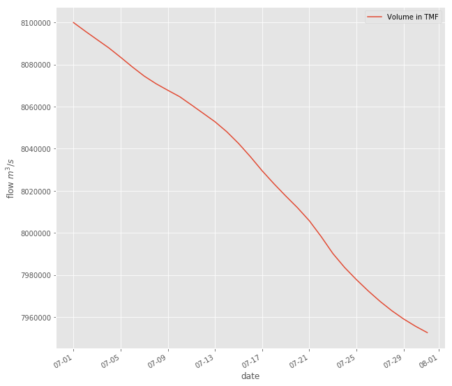
[8]:
# # in second plot, plot the volume in TMF in m^3, which is stored in the "volume" column
plt.plot(df_flow["yearmonthday"], df_flow["volume"], label="Volume in TMF")
plt.legend()
ax = plt.gca()
fig = plt.gcf()
ax.set(ylabel="flow $m^3/s$", xlabel="date")
ax.xaxis.set_major_formatter(myFmt)
fig.autofmt_xdate()