1. Understanding the greenhouse effect

• Presentation by Phil Austin, 2023/May/31

  • Web version: https://phaustin.github.io/climatemath/docs/greenhouse.html

  • Repository: phaustin/climatemath

1.1. Big picture

The greenhouse effect is the change in longwave radiation escaping to space due to the presence of an atmosphere.

(Note that this doesn’t have much to do with actual greenhouses)

It depends on the vertical profiles of the absorptivity and temperature of the greenhouse gas (and liquid and ice particles, if we’re considering clouds).

1.1.1. A specific example – the Earth’s current atmosphere

GH = -239 \(W\,m^{-2}\) - (-398) \(W\,m^{-2}\) = 159 \(W\,m^{-2}\)

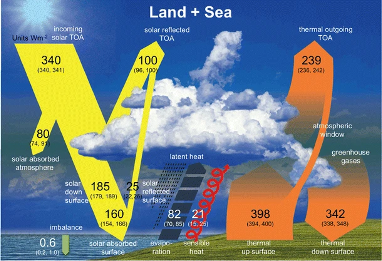
Fig. 1.1 Estimated energy fluxes, current climate

1.1.2. Important points:

• The atmosphere absorbs and emits longwave radiation.

• Increasing greenhouse gas concentration increases the emissivity of the atmosphere (note the contradiction with Homework 1 ). There is an important distinction between emission (net emitted flux in \(W\,m^{-2}\)) and emissivity (unitless, the relative ability of a gas molecule to emit a photon compared to a blackbody)

• To first order, absorption is independent of temperature, while emission is a strong function of temperature

• Because the atmosphere is colder than the surface, it absorbs radiation from the surface and emits less radiation to space. Increasing emissivity decreases emission because it moves the emission layer to higher altitudes/colder temperatures.

• This reduction in surface radiative cooling by the atmosphere is the atmospheric greenhouse effect.

• Any successful theory of the the anthropogenic greenhouse has to explain both tropospheric warming and stratospheric cooling

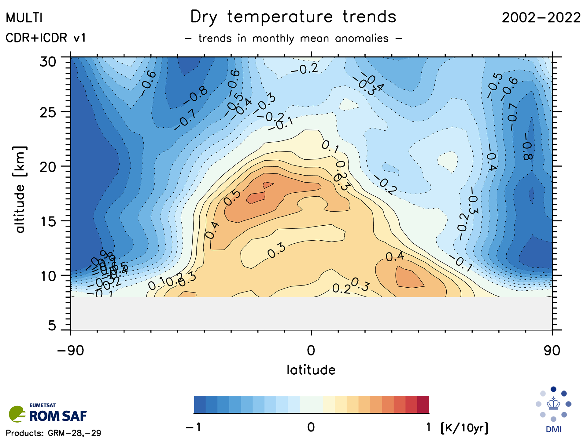
Fig. 1.2 Decacal temperature trends (K/decade) between 2002-2022

1.2. Outline

3. Basic concepts

• Flux and radiance, Planck’s law, Beer’s law and Kirchoff’s law, optical depth

4. The single layer greenhouse

• Simple model of an absorbing and emitting atmosphere over a black surface

5. Wavelength dependent emissivity

• Absorption spectra for greenhouse gasses

6. The Schwarzchild equation for radiance

• Governing ode for absorption and emission

7. Weighting functions, emission level and the greenhouse effect

• The link between \(CO_2\) concentration, photon emission level and the greenhouse effect

8. The Schwarzchild equation for flux

• Integrating the radiance to calculate the upward flux

9. Tropospheric warming and stratospheric cooling

• Calculating the impact of the temperature profile on the greenhouse effect

• Introduce a notebook to solve the Schwartzchild equation for realistic atmospheres

10. Summary

1.3. Basic concepts

1.3.1. Planck’s law

• Electromagnetic emission obeys Planck’s law:

(1.1)\[ B_\lambda(\lambda, T)=\frac{2 h c^2}{\lambda^5} \frac{1}{e^{h c /\left(\lambda k_{\mathrm{B}} T\right)}-1} \]

where \(T\) is temperature, \(\lambda\) is wavelength, \(k_B\) is Boltzman’s constant, \(h\) is Planck’s constant and \(c\) is the speed of light.

\(B_\lambda\) is called the “monochromatic blackbody radiance”, and has units of \(W\,m^{-2}\,\mu m^{-1}\,sr^{-1}\) (in words: Watts per square meter per micron bin width per steradian field of view)

Integrating (1.1) over all wavelengths yields the Stefan-Boltzman equation for flux:

(1.2)\[ \int_0^\infty B_\lambda(\lambda, T) d\lambda = \frac{\sigma}{\pi} T^4\ (W\,m^{-2}) \]

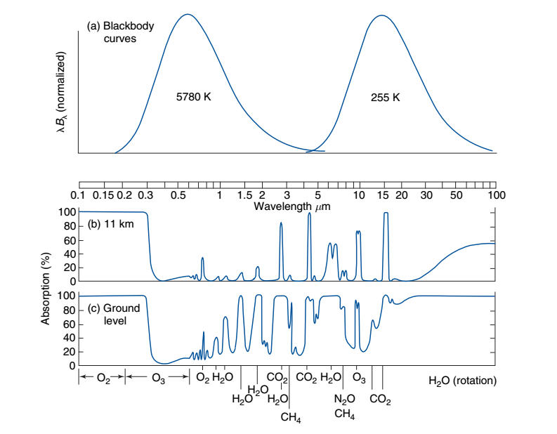
Fig. 1.3 Selective absorption by greenhouse gases. Note the 15 \(\mu m\) \(CO_2\) band coincides with the Planck peak emission at 255 K.

1.3.1.1. Sample Problems

1. Use change of variables to rewrite (1.1) in terms of wavenumber \(\tilde{\nu} = 1/\lambda\) and show that it is:

(1.3)\[ B_{\tilde{\nu}}(\tilde{\nu}, T)=2 h c^2 \tilde{\nu}^3 \frac{1}{e^{h c \tilde{\nu} /\left(k_{\mathrm{B}} T\right)}-1} \]

2. Integrate (1.3) to find the Stefan-Boltzman equation given that

(1.4)\[ \int_0^\infty \frac{u^3}{(e^u -1 )} du = \frac{\pi^4}{15} \]

(Riemann zeta function)

3. Show that the maximum value for (1.1) occurs at:

\[ \lambda_{max} \propto \frac{1}{T} \]

(Wien’s law)

1.3.2. Definition: flux

• Flux density (or irradiance)

  Units: \(W\,m^{-2}\)

  Definition: electromagnetic energy passing through unit area in unit time

  Symbol: E

  (for physicists – we’re talking about \(S\), the Poynting vector )

  Not conserved in a vacuum – flux decreases as \(1/\text{distance}^2\)

• Some assumptions for undergraduates

  • Shortwave flux: all photons with wavelengths \(\lt\) 4 \(\mu m\) are emitted by the sun

  • Shortwave flux: neglect absorption

  • Longwave flux: all photons with wavelengths \(\gt\) 4 \(\mu m\) are emitted by terestrial solids, fluids or gasses

  • Shortwave flux from the sun (the direct beam) is directional/collimated, scattering dominates

  • Longwave flux is isotropic, scattering is negligible

1.3.3. More useful for radiative transfer: radiance

The flux has two undesirable properties:

• Not easy to measure directly (because no instrument can sample over a complete hemisphere)

• Isn’t conserved in a vacuum (decreases with distance R from the emitter as \(1/R^2\))

Satellites/telescopes measure the radiance

• Radiance

  Units: \(W\,m^{-2}\,sr^{-1}\)

  Definition: electromagnetic energy passing though unit area in unit time in unit field of view

  Symbol: L

  Conserved in a vacuum

1.3.3.1. Sample problem: Relate the radiance and the flux

We can integrate the normal component of the radiance over a hemisphere to get the flux

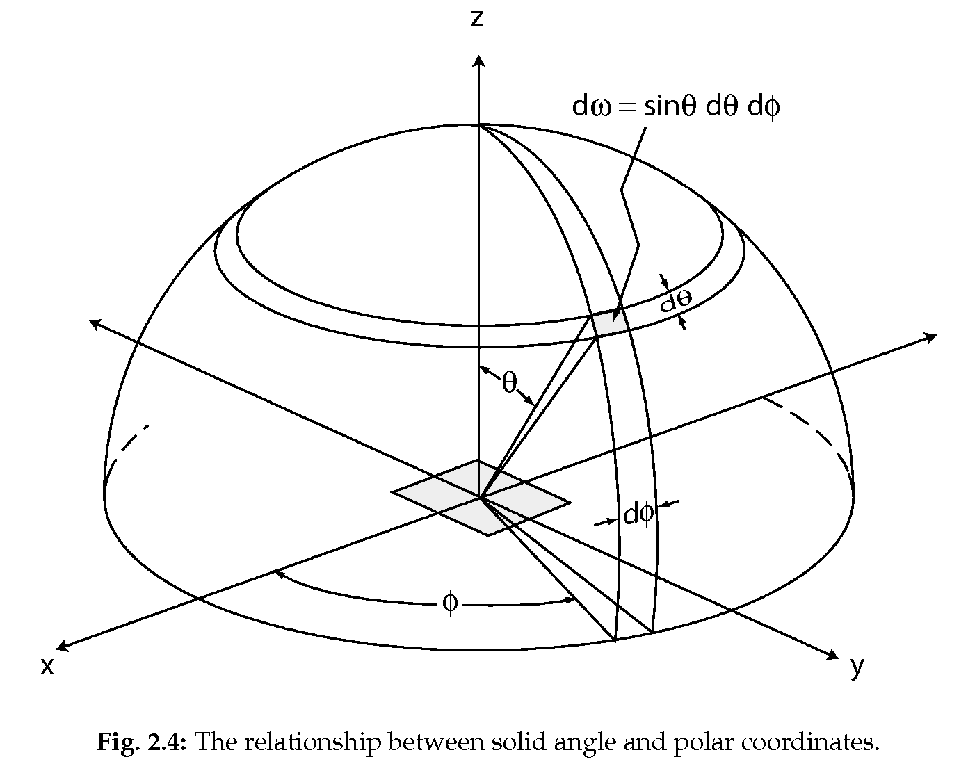
Consider an instrument on the ground looking upward with a limited field of view \(d\omega\). At radius \(r\) the telescope is subtending an area \(dA\) where:

\[ dA = width \times height = R \sin \theta d\phi \times r d\theta = R^2 \sin \theta d\theta d \phi \]

(1.5)\[ d\omega = \frac{dA}{R^2} = \frac{R^2 \sin \theta d\theta d\phi}{R^2} = \sin \theta d\theta d\phi \]

It’s common to do a change of variables:

\[ \mu = cos\theta \]

(1.6)\[ d\omega = \frac{dA}{R^2} = \frac{R^2 \sin \theta d\theta d\phi}{R^2} = \sin \theta d\theta d\phi = -d\mu d\phi \]

So the flux \(dE\) reaching the telescope sensor from that field of view is the normal component of \(L d\omega\):

\[ dE = \int_{\phi_1}^{\phi_2} \int_{\mu_1}^{\mu_2} \cos \theta L d\mu d\phi = \int_{\phi_1}^{\phi_2} \int_{\mu_1}^{\mu_2} \mu L d\mu d\phi \]

If the radiance is isotropic (say we are hovering close to the ocean surface, looking downward, or orbiting a planet without an atmosphere), then the total flux is just:

\[ E = L \int_{0}^{2 \pi} \int_{0}^{1} \mu d\mu d\phi = 2 \pi \frac{\mu^2}{2} L = \pi L \]

Note: this is why there is a factor of \(1/\pi\) in (1.2).

Question: Why doesn’t the perceived brightness of a piece of white paper obey the inverse-square law for flux?

1.3.4. Beer’s law: Transmission and absorption of radiance

Given the radiance, we can write a differential equation to describe absorption by a greenhouse gas.

We define the “absorptivity” \(a\) for a greenhouse gas as

\[ a = \frac{dL}{L} \]

Fig. 1.4 illustrates the two quantities we need to quantify the absorptivity: \(ds\) (m) is the slant path and \(\sigma\) (\(m^2\,m^{-3}\)) is the volume absorption coefficient.

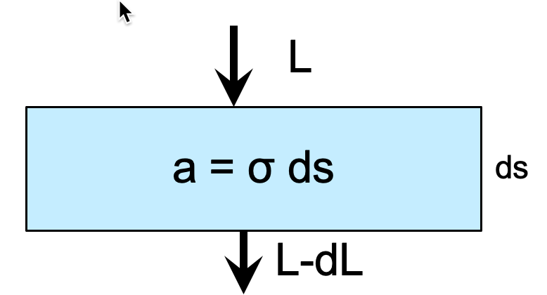
Fig. 1.4 An atmospheric layer with absorptivity \(a\)

Beer’s law (really Maxwell’s equations) states that:

(1.7)\[ dL = -L \sigma ds = -L d\tau \]

where we’ve introduced a new variable, the \(\tau = \int \sigma ds\), the optical depth.

Integrating equation (1.7) yields the transmissivity for the layer:

(1.8)\[ t_r = L/L_0 = \exp(-\tau) \]

The optical depth is the fundamental scaling property for a radiating atmosphere.

1.3.5. Conservation of energy

An additional constraint is that every photon must be absorbed, transmitted or reflected. Recall that we’re neglecting reflection in the longwave, so the energy constraint is:

(1.9)\[ t_{r\lambda} + a_\lambda = 1 \]

Taking the differential of (1.9):

(1.10)\[ dt_{r \lambda} = -da_\lambda = -d\tau_\lambda \]

1.3.6. Sample problem: Relating the volume absorption coefficient \(\sigma\) to the mean free path

How far can a photon travel before it’s absorbed?

The probability that an absorption event will occur in distance \(d s\) is just the fraction of photons that make it through \(ds\) without being absorbed:

\[ p(s)\,ds = \exp(-(\sigma \,s)) - \exp(-(\sigma (s + ds )) \]

take the limit to get the PDF for an absorption event:

\[ p(s)= \frac{d \exp(-(\sigma \,s)) }{ds} = -\sigma \exp(-(\sigma s)) \]

The first moment of \(p(s)\) is the mean distance traveled before an absorption:

\[ \langle s \rangle = \int_0^\infty\, s \, p(s)\,ds = \int_0^\infty s\ \exp(-\sigma s)\, ds = \frac{1}{\sigma} \]

So the volume absorption coefficient is the inverse of the average distance a photon travels from emission to absorption

1.3.7. Kirchoff’s law: \(a_\lambda = \epsilon_\lambda\)

“Good absorbers are good emitters”

As the transmissivty plots in Fig. 1.3 indicate, greenhouse gasses are extremely selective absorbers. An important result from statistical mechanics: any gas in local thermodynamic equilibrium at temperature T that is absorbing radiation at wavelength \(\lambda\) will be emitting radiance

\[ L_{emitted} = \epsilon_\lambda B_\lambda(\lambda, T) \]

Where \(\epsilon_\lambda\) is the monochromatic emissivity (unitless).

Fig. 1.5 below shows why \(\epsilon_\lambda = a_\lambda\) in a collision dominated system. Since the plates are horizontally infinite, the gas is absorbing flux \(2 a_\lambda \pi B(\lambda, 300)\) from the black plates, and emitting \(2 \epsilon_\lambda \pi B(\lambda, 300)\) back to the plates. If \(a_\lambda \neq \epsilon_\lambda\), the temperature of the gas would change, violating the 2nd law of thermodynamics.

\[\begin{split} \begin{align} 2 a_\lambda \pi B(\lambda, 300) &= 2 \epsilon_\lambda \pi B(\lambda, 300)\\ a_\lambda &= \epsilon_\lambda \end{align} \end{split}\]

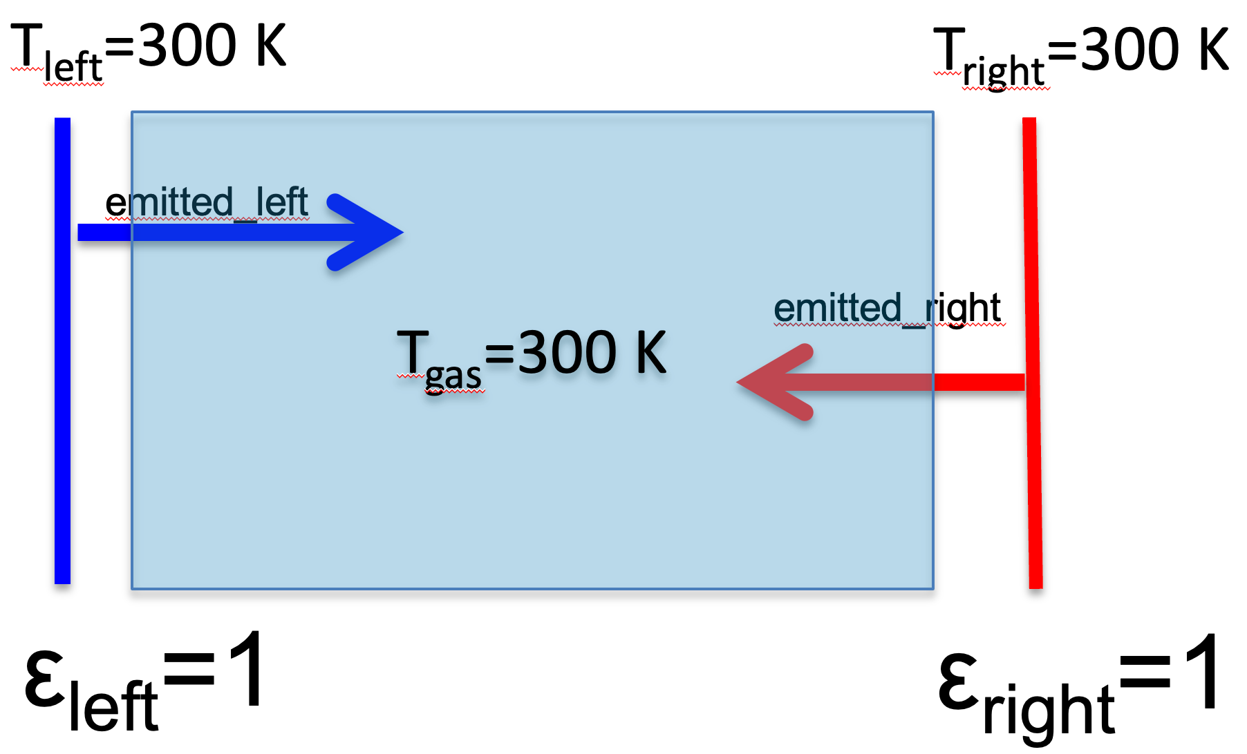
Fig. 1.5 A greenhouse gas with aborptivity \(a_\lambda\) and emissivity \(\epsilon_\lambda\) between two black plates

Using (1.10) we also have for the differentials:

(1.11)\[ da_\lambda = d\epsilon_\lambda = d\tau_\lambda \]

1.3.8. Summary

• The optical depth \(\tau\) scales the change in absorption and emission in the atmosphere

• \(\tau\) is a very strong function of wavelength, due to the wavelength dependence of the volume absorption coefficient

• \(d\tau\) is closely related to the mean free path, transmissivity, absorptivity of thin atmospheric layers

• Given an optical depth profile, Beer’s law predicts the path dependent absorption of incident radiation

1.4. A single-layer model of the greenhouse effect

Fig. 1.6 below shows how \(\epsilon\) is related to the upward and downward fluxes in an atmosphere overlying a black absorbing surface. Note that due to Kirchoff’s law, \(\epsilon\) is representing both the emissivity and the absorptivity/transmissivity of the layer.

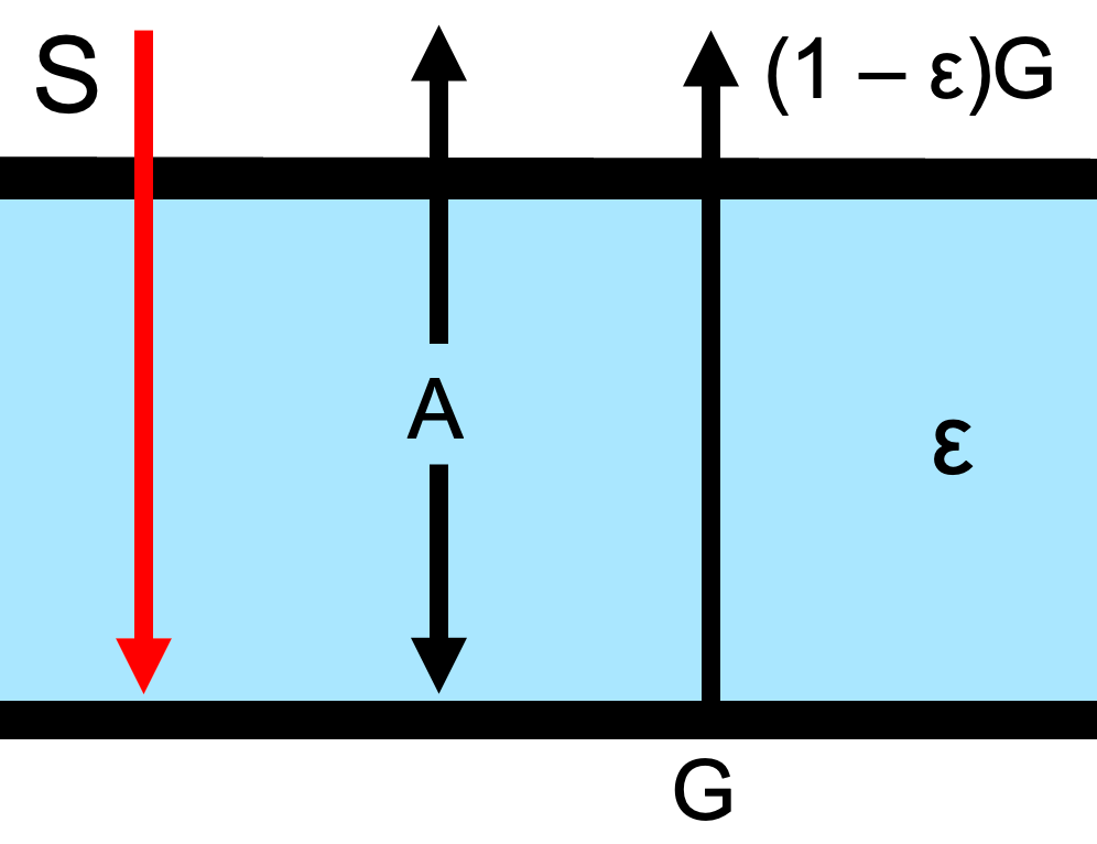
Fig. 1.6 An atmospheric layer with emitted flux with emissivity/absorptivity \(\epsilon\), emitted flux \(A\), incoming shortwave flux \(S\) and upwelling flux from below \(G\)

In equilibrium, the net flux has to be zero at both top and bottom boundaries.

Solving for the unknown fluxes \(A\) and \(G\) gives:

(1.12)\[ A = \frac{\varepsilon S}{\left( 2 - \varepsilon \right)} = \varepsilon \sigma T_{A}^{4} \]

\[G = \frac{2S}{\left( 2 - \varepsilon \right)} = \sigma T_{G}^{4}\]

and rearranging:

(1.13)\[ T_A = \sqrt[4]{\frac{S}{(2 - \varepsilon) \sigma}} \]

(1.14)\[ T_G = \sqrt[4]{\frac{2 S}{(2 - \varepsilon) \sigma}} \]

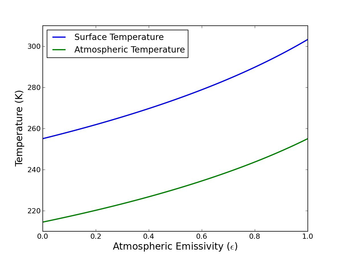
Fig. 1.7 An atmospheric layer with emitted flux with emissivity/absorptivity \(\epsilon\), emitted flux \(A\), incoming shortwave flux \(S\) and upwelling flux from below \(G\)

1.4.1. Sanity Check: average emissivity at current solar constant S

For current solar output and a planetary reflectivity of 30%, \(S=240\ W\,m^{-2}\). With this solar constant (1.14) gives a surface temperature of 287 K (the current global average) with an emissivity of \(\epsilon = 0.75\)

This isn’t too far from the approximate observed average longwave emissivity of 0.8.

S=240
sigma = 5.67e-8
eps = 0.75
Tg = (2*S/((2 - eps)*sigma))**0.25
Ta = (S/((2 - eps)*sigma))**0.25
print(f"{Tg=:.0f} K, {Ta=:.0f} K")

Tg=287 K, Ta=241 K

1.4.2. Thin layer limit: The skin temperature is independent of \(\epsilon\)

If we change the interpretation of the flux G in Fig. 1.6 to be the total upward flux from the surface and lower atmosphere, then we can find the “skin temperature” at the top of the atmosphere by taking the thin layer limit \(\epsilon \rightarrow 0\) in (1.12) and get

(1.15)\[ T_{skin} = \sqrt[4]{\frac{S}{2 \sigma}} \]

Putting \(S=240\ W\,m^{-2}\) into (1.15) yields \(T_{skin}\) = 214 K, independent of the greenhouse gas concentration. This is a good approximation to observed atmospheric temperatures at the tropopause.

Tskin = (S/(2*sigma))**0.25
print(f"{Tskin=:.0f} K")

Tskin=214 K

1.4.3. Summary

• A single layer model of an equilibrium atmosphere is consistent with both the observed surface and atmospheric temperatures

• The skin temperature of the top of the atmosphere depends only on the net downward shortwave flux. This is because absorptivity and emissivity have to balance in the layer.

• Greenhouse gasses at the top atmosphere absorb much more than they emit. This energy is mixed throughout the atmospheric column by convection

1.5. Calculating the wavelength-dependent emissivity of a greenhouse gas

In Section 1.4 we found a wavelength-averaged \(\epsilon\) consistent with current \(S\) and surface temperature. To move further, we need to link \(\epsilon_\lambda\) to the volume absorption coefficient \(\sigma_\lambda\) for the greenhouse gas. To do this first decompose \(\sigma_\lambda\) into two components: The absorber gas density \(\rho_{gas}\ (kg\,m^{-3})\), and the mass absorption coefficient \(k_\lambda\ (m^{2}\,kg^{-1})\)

\[ \sigma_\lambda = \rho_{gas} k_\lambda \]

How do we calculate \(k_\lambda\)? There are absorption coefficient databases that provide “line by line” \(k_\lambda\) values for individual energy level transitions.

These absorption lines are then parameterized for use in variety of radiative transfer models like Modtran

1.5.1. Three \(CO_2\) absorption lines

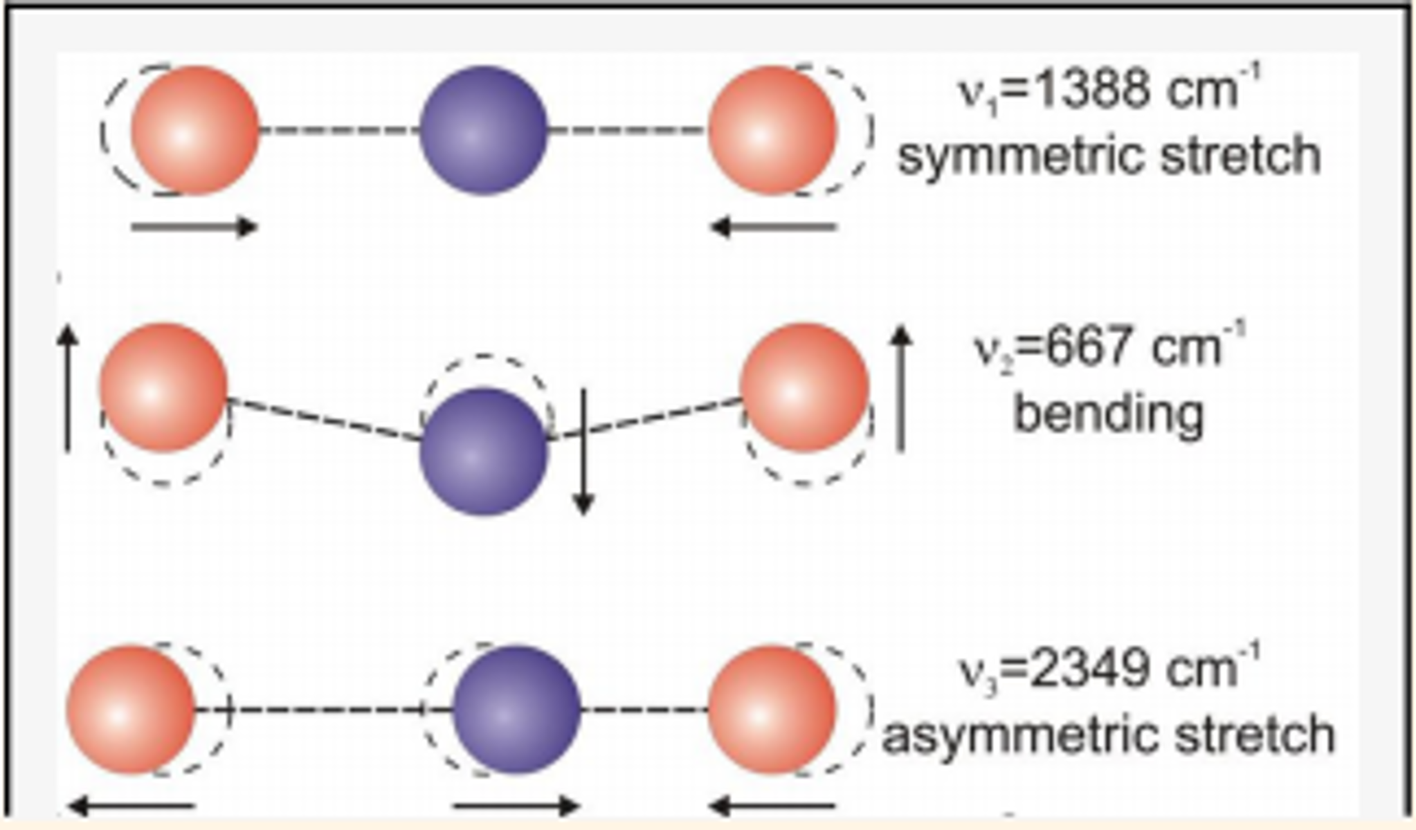
Fig. 1.8 Three \(CO_2\) absorption lines: 7 \(\mu m\), 15 \(\mu m\), and 4.3 \(\mu m\)

1.5.2. Full spectra for 3 greenhouse gasses

Note that in the \(CO_2\) band between 550-700 \(cm^{-1}\) (14-18 \(\mu m\)) \(k_\lambda\) varies by about 5 orders of magntude.

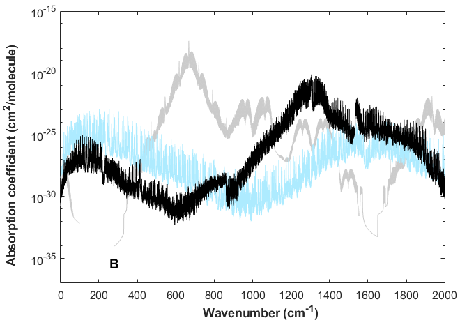
Fig. 1.9 \(k_\lambda\) spectrum for \(CO_2\) (gray), \(CH_4\) (black), \(H_2O\) (grey).

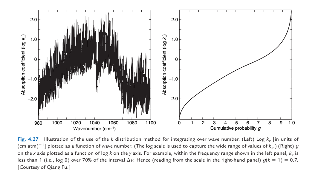
1.5.3. Aside: Lebesgue integration for climate model parameterizations

Global climate models parameterize the wavelength, temperature and pressure dependence of the various absorption bands using the “correlated-k” approximation, which is a variant of Lebesque integration. It reduces the number of quadrature points needed to integrate absorption bands by 4-5 orders of magnitude.

1.5.4. Summary

• The relationship between the emissivity and the greenhouse gas concentration is well-understood both theoretically and experimentally

• The volume scattering coefficent, and therefore the optical depth, is a function of gas concentration and absorption line strength, which in turn depends on wavelength, temperature, and atmospheric pressure.

• Getting accurate heating and cooling rates in climate models is non-trivial, but essentially a solved problem.

1.6. The Schwarzchild equation for radiance

gUsing (1.11) we can add an emission term to (1.7) to get the Schwarzchild equation for vertical radiance:

\[ dL = -L\,d\tau + B\,d\tau \]

Choose a coordinate system where \(\tau\) is zero at the top of the atmosphere increasing downwards:

\[ \tau = \int_z^\infty \rho_{gas} k_\lambda dz \]

Use an integrating factor:

(1.16)\[ \exp(\tau) dL + L \exp(\tau)\,d\tau=\exp(\tau)B_\lambda(T) \,d\tau \]

Impose boundary conditions and integrate from the top of the atmoshere down to optical depth \(\tau_{\lambda T}\) to get the upward radiance at the top of the atmosphere, where \(\tau = 0\):

(1.17)\[ L(0)= B_\lambda(T_{sfc}) \exp(-\tau_{\lambda T}) + \int_0^{\tau_{\lambda T}} \exp\left(-\tau^\prime \right ) B_\lambda(T)\, d\tau^\prime \]

Since the transmission is defined as \(t_r = \exp(-\tau)\), we can change variables and write:

(1.18)\[ L(0) = B_\lambda(T_{sfc})t_{rtot} + \int_{t_{rtot}}^{1} B_\lambda(T)\, dt_r^\prime \]

1.6.1. Sample problem

Use the mean value theorem to show that there is an average temperature \(\hat{T}\) that allows us to write (1.18) in the form:

\[ L(0) = B_\lambda(T_{sfc})t_{rtot} + (1 - t_{rtot})B_\lambda(\hat{T}) \]

and that this corresponds to the situation depicted in Fig. 1.6.

1.6.2. Summary

• The Schwarzchild equation is a first-order ode that predicts the radiance along a path as a function of gas temperature and gas absorption

• To be usefull in climate model calculations, a model has to integrate a solution along the absorber path, over all wavelengths and over a hemisphere to get the radiative flux passing through a model layer

1.7. Weighting functions

We can get some more insight into how absorption and transmission work by rewriting (1.18) as folows:

\[\begin{split} \begin{align} L(0) &= B_\lambda(T_{sfc})t_{rtot} + \int_{t_{rtot}}^{1} B_\lambda(T)\, dt_r^\prime \\ &= B_\lambda(T_{sfc}) t_{rtot} + \int_0^{z_{top}} B_\lambda(T)\, \frac{dt_r}{dz^\prime} dz^\prime \end{align} \end{split}\]

The derivative \(dt_r/dz\) is called the weighting function and determines the relative contribution of the thermal emission of each layer to the upwelling radiance leaving the atmosphere.

For a “well-mixed” absorber like \(CO_2\), in which the absorber mass fraction is constant with height, the absorber density has an exponential profile:

\[ \rho_{gas}(z) = \rho_0 \exp(-z/H) \]

where \(H\) is the scale height for the absorber.

Integrating the optical depth for that case gives:

(1.19)\[ \tau(z) = \int_{z}^{\infty} \rho_{gas} k_\lambda dz^\prime = H k_\lambda \rho_0 \exp(-z/H) \]

1.7.1. Sample problem

Insert (1.19) into (1.8) and differentiate twice to show that the maximum values of the weighting function \(dt_r/dz\) occurs at \(\tau = 1\)

1.7.2. Figure examples

Fig. 1.10 below shows a weighting function \(dt_r/dz\) (short-dashed line)for this case.

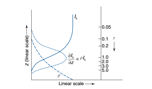
Fig. 1.10 Vertical transmissivity (\(I_\lambda\) in this book’s notation) as a function of height.

Fig. 1.11 below shows the actual weighting functions and transmissivty profiles for a satellite radiometer that measures the vertical temperature profile using the 15 \(\mu m\) \(CO_2\) band. Channels 1, 2, and 3 are measuring photons predominantly emiited from the stratosphere, while channels 4, 5 and 6 are measuring tropospheric emission.

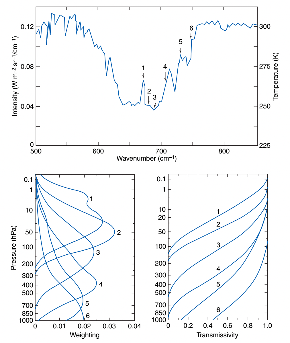
Fig. 1.11 \(CO_2\) weighting functions and transmissivity for a satellite sounder

Note that this is how the temperature retrievals were made in Fig. 1.2

1.7.3. Summary

• The weighting function selects the portion of the atmosphere that contributes most to outgoing emitted radiation to space.

• As the optical depth increases at a particular wavelength (because of increased \(CO_2\) concentration), the altitude of maximum emission increases.

• In the troposphere, the temperature decreases with altitude, so emission at that wavelength will decrease, increasing the greenhouse effect.

1.8. The Schwarzchild equation for flux

So far we’ve restricted ourselves to a single vertical direction, and calculated the radiance along the vertical slant path \(s=z\). If we want to integrate over a hemisphere to get the flux, we’re going to need to sample all angles, which means all slant paths \(s = z/\cos \theta = z/\mu\)

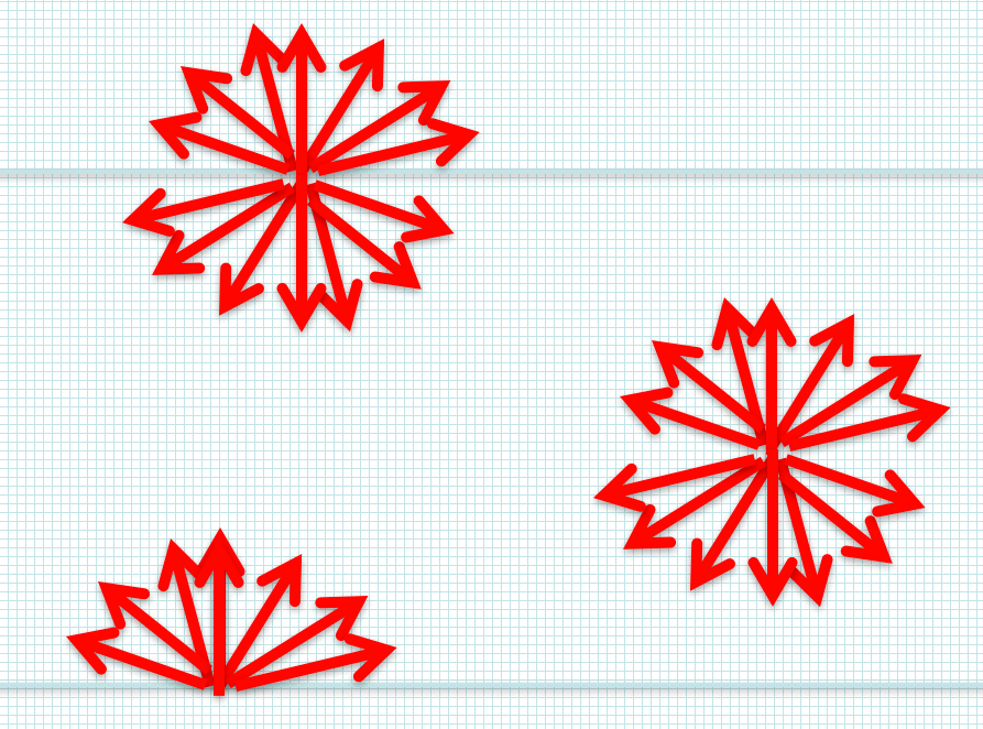
Fig. 1.12 Slant paths for thermal emission

1.8.1. Slant path transmissivity

The slant path version of (1.17):

(1.20)\[ L(0,\mu)= B_\lambda(T_{sfc}) \exp(-\tau_{\lambda T}/\mu) + \int_0^{\tau_{\lambda T}} \exp\left(-\tau^\prime /\mu\right ) B_\lambda(T)\, \frac{d\tau^\prime}{\mu} \]

Assume azimuthal isotropy so we can integrate out \(\int_0^{2\pi} d\phi = 2\pi\). Then we’re left with:

(1.21)\[\begin{split} \begin{align} E(0) &= 2\pi \int_0^1 \mu L(0,\mu) d\mu \\ & 2 \pi \int_0^1 \mu B_\lambda(T_{sfc}) \exp(-\tau_{\lambda T}/\mu) d\mu + 2 \pi \int_0^1 \int_0^{\tau_{\lambda T}} \mu \exp\left(-\tau^\prime /\mu\right ) B_\lambda(T)\, \frac{d\tau^\prime}{\mu} d\mu \end{align} \end{split}\]

The Planck function is isotropic so can be taken out of the \(\mu\) integral, so define the flux transmission:

(1.22)\[ \hat{t}_f = 2 \int_0^1 \mu \exp \left (- \frac{\tau }{\mu} \right ) d\mu \]

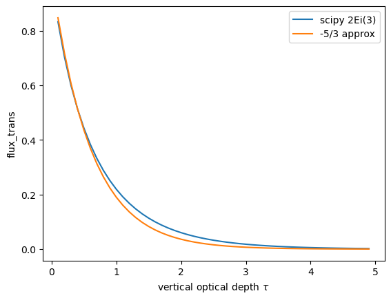
Make the change of variables \(u = \mu^{-1}\) to get the third exponential integral:

\[ \hat{t}_f = 2 \int_1^\infty \frac{\exp(-u \tau)}{u^3} du = 2E_i(\tau) \]

which is available from scipy as expn(3.0, tau). Luckily, to a pretty good approximation we can fake the integration by just multiplying the optical depth by 5/3. This is called the diffusivity approximation

(1.23)\[ \hat{t}_f = 2 \int_1^\infty \frac{\exp(-u \tau)}{u^3} du = 2E_i(\tau) = \exp(-1.66 \tau) \]

The python code below compares \(\exp(-1.66 \tau\) with \(2E_i(\tau)\). The approximation is very good for \(\tau < 1\).

from matplotlib import pyplot as plt
import numpy as np
from scipy.special import expn
tau = np.arange(0.1, 5, 0.1)
flux_trans = 2 * expn(3.0, tau)
fig, ax = plt.subplots(1, 1)
ax.plot(tau, flux_trans, label="scipy 2Ei(3)")
ax.plot(tau, np.exp(-1.66 * tau), label="-5/3 approx")
ax.legend()
ax.set(ylabel="flux_trans", xlabel=r"vertical optical depth $\tau$");

1.8.2. The Schwarzchild equation under the diffusivity approximation

Using the diffusivity approximation, (1.21) can be rewritten as:

(1.24)\[ \begin{align} E(0) = \underbrace{\pi B_\lambda(T_{sfc}) \hat{t}_{ftot}}_{\text{transmission}} + \underbrace{\pi \int_{\hat{t}_{ftot}}^1 B_\lambda(T) d\hat{t}_f}_{emission} \end{align} \]

which is a close parallel to the radiance equation (1.18).

1.8.3. Summary

• Thanks to the diffusivity approximation it is relatively easy to account for the impact of slant paths on radiation transport between vertical levels

1.9. Tropospheric warming and stratospheric cooling

Recall from Fig. 1.2 that we are seeing warming in the troposphere and cooling in the stratosphere

To get the greenhouse effect from (1.24), we need to subtract the surface flux:

\[\begin{split} \begin{align} GH_\lambda &= \pi B_\lambda(T_{sfc}) - E(0) = \pi B_\lambda(T_{sfc}) ( 1 - \hat{t}_{ftot} ) - \pi \int_{\hat{t}_{ftot}}^1 B_\lambda(T) d\hat{t}_f\\ &= \pi B_\lambda(T_{sfc}) ( 1 - \hat{t}_{ftot} ) - \pi B_\lambda(\hat{T})(1 - \hat{t}_{ftot}) \end{align} \end{split}\]

To see why increasing greenhouse gasses cools the statosphere, note that in the stratosphere, \(B_\lambda(T_{sfc}) < B_\lambda(\hat{T})\). As \(CO_2\) concentration increases, the flux transmissivity \(\hat{t}_{ftot}\) decreases. With the temperature increasing with height, the result will be a net negative change in the greenhouse effect.

1.10. Conclusions

1.10.1. Greenhouse physics

1. Greenhouse gases selectively absorb and emit longwave photons in discrete bands.

2. The earth cools by emission of longwave photons to space.

3. The height at which this emission occurs depends on the photon wavelength and the molecular structure and concentration of the greenhouse gas. It is set by the atmospheric level at which the optical depth \(\tau = 1\). This level is high in the atmosphere for strong absorbing bands, and lower in the atmosphere for weaker bands.

4. The gas temperature decreases with height in the toposphere (because thermal energy is used to lift the atmosphere above the surface)

5. The gas temperature increases with height in the stratosphere (because ozone absorbs hard ultraviolet radiation)

6. We are increasing the greenhouse gas concentration, and therefore moving the emission altitude higher for all absorption bands

7. In the troposphere, this produces reduced emission to space from colder temperatures, heating the atmosphere

8. In the startosphere, this produces increased emission to space, cooling the stratosphere.

1.10.2. Math concepts

1. Integrals and derivatives – e.g. (1.19), Section 1.7

2. Spherical coordinates, solid angle: (1.6)

3. Working with differentials/Taylor series – e.g.:

   \[dt_r = d\exp(-\tau) = -\exp(-\tau)\,d\tau \approx -d\tau\]

4. Change of variables – e.g.: (1.3)

5. ODEs/integrating factors – e.g. (1.17)