Table of Contents
1 Learning goals
2 Approach to develop a partial differential equation
2.1 2-d transient mass - balance statement
2.2 Sign conventions
2.3 Upshot
2.4 Per unit volume, per unit time
2.5 Your turn
2.6 Partial differential equation
3 Conservation of mass equation in 3 dimensions
3.1 Interpretation
3.2 Your turn
3.3 Divergence of a vector
3.4 Your turn
4 Vector notation
4.1 Why \(\vec{\nabla}\)?
5 Diffusion equation
5.1 Your turn
5.2 Constant diffusion coefficient
5.3 Diffusion in porous media
5.4 For homogeneous porosity
6 Solving PDEs: Boundary - value problems
6.1 Boundary-value problem checklist
6.2 TMF BVP example
6.3 Equation
6.4 Domain
6.5 Properties of the problem domain
6.6 Boundary conditions
6.7 Initial conditions
7 Assignment
8 1 Finding an analytical solution
8.1 Your turn
9 2 Interpretation
9.1 1.
9.2 2.
9.3 3.
9.4 4.
Learning goals
Be able to take a discrete approximation to limit of infinitesimal volume size and time step to arrive at the partial differential equation.
Be able to read a partial differential equation:
distinguish between terms that represent fluxes, sources and storage of quantities within the volume (infinitesimal point).
recognize the order of the equation.
recognize conservative forms
Be able to simplify a partial differential equation when coefficients are constant.
Recognize the conservation principle in integral form and match it to the corresponding partial differential equation.
Be able to set up boundary value problem:
define domain of the problem.
define the equations that govern the dependent variable.
define the parameters of the equation, and if they are spatially homogeneous (do not vary in space) or heterogeneous.
distinguish between the principal boundary conditions that prevail.
assign initial conditions (if a time dependent problem).
Be able to understand the significance of the mathematical concept of divergence and its relationship to flux at a point.
Be able to recognize a partial differential equation when written in vector form using divergence and gradient.
Approach to develop a partial differential equation
Write a discrete approximation for mass conservation for a finite volume.
Take limits as the size of the volume element and the time period of consideration shrink to infinitesimal size.
Recognize limits as derivatives. Where the independent variable (eg concentration) is a function of more than one dependent variable (typically 3 space dimensions \(x\), \(y\) and \(z\), and \(t\)), the derivatives are partial.
[1]:
from IPython.display import Image
[2]:
Image("figures/shrink_to_infinitesimal.png", width="35%")
[2]:

2-d transient mass - balance statement
We’ll do this in 2-d. From that we can easily go to either 3-d or 1-d.
We’ll consider the transient case, where mass is changing in time in the volume. Let’s consider the simple 2-d stencil, where the gridblock is of size \(\Delta x\), \(\Delta y\), \(\Delta z\) (where \(\Delta z\) is into the page in the figure below).
[3]:
Image("figures/nsewc_stencil.png", width="20%")
[3]:
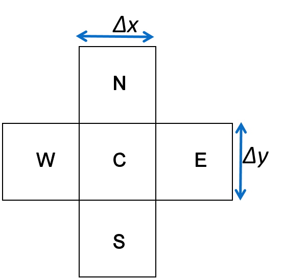
Recall from notebook 5.1_finite_volume_2.ipynb A transient conservation statement is * the change of the quanity in the volume over a time :math:`Delta t` = the net flux of the quantity into the volume over the time period :math:`Delta t`.
To make things more concrete, let’s consider the case where the conserved quantity is mass \(m\), such as sulfate.
In one dimension, the transient conservation expression is (from 5.1_finite_volume_2.ipynb):
\begin{align} \Delta m_C = m_C(t+\Delta t) - m_C(t) & = (J_E+J_W)\Delta t \label{1dcons}\\ \end{align}
where both sides of the equation have dimensions of mass: * \(m_C(t)~\left[M\right]\) is the mass in gridblock C at time \(t\) and \(m_C(t+\Delta t)~\left[M\right]\) is the mass in gridblock C at time \(t+\Delta t\) * \((J_E+J_W)\Delta t~\left[M\right]\) is the net mass that fluxed into volume over time period \(\Delta t\).
If we now go to 2-d and express this equation in terms of specific fluxes \({j}\), and recall that \({J}=jA\) where we multiply the net specific flux by the area of the boundary of volume perpendicular to the flux component (eg for fluxes in the \(x\) direction, the area perpendicular is \(\Delta y \Delta z\)): \begin{align} \left(m_C(t+\Delta t) - m_C(t)\right) = \left\{\left(j_{EC} + j_{WC}\right) \Delta y \Delta z + \left(j_{NC} + j_{SC}\right) \Delta x \Delta z \right\}\Delta t \label{7pde1}\\ \end{align}
Sign conventions
The next step is to re-express the fluxes in the discrete approximation such as \(j_{EC}\) in terms of components of a flux vector that varies continuously with location (here in 2-d) \(\vec{j}= \left\{j_x, j_y\right\}\) - the “true” flux that is approximated at gridblock edges by \(j_{EC}\), etc. The only “trick” here is to be careful of the sign conventions.
In contrast to our finite volume convention where fluxes such as \(j_{EC}\) are positive for flux into the volume, in math, a vector component is positive if the vector is pointing in the direction in which the coordinate direction corresponding to that component is increasing.
We’ll demonstrate this for the \(x\) direction here. Consider gridblock C where the left (W) face is located at \(x\) and the right (E) face is located a position \(x+\Delta x\). First, recognize that both \(j_{WC}\) and \(j_{EC}\) are \(x\) flux components.
Here is the correspondence:
\(j_{WC}\) corresponds to \(j_x(x,y,z)\) because when \(j_x\) is positive, flux enters C, just like \(j_{WC}\)
\(j_{EC}\) corresponds to \(-j_x(x+\Delta x,y,z)\) because when \(-j_x\) is positive flux enters C, just like \(j_{EC}\)
Example, for some hypothetical situation, \(j_x(x,y,z) = 3~mg/(s\cdot m^2)\) and \(j_x(x+\Delta x,y,z) = -2.5~mg/(s\cdot m^2)\), then * on the W face, \(j_x\) is directed in the positive \(x\) direction, so is flowing into C, so \(j_{WC} = j_x(x,y,z) = 3~ mg/(s\cdot m^2)\) * on the E face, \(j_x\) is directed in the negative \(x\) direction, so is flowing into C, so \(j_{EC} = -j_x(x+\Delta x,y,z) = 2.5 ~mg/(s\cdot m^2)\)
Upshot
In our conservation statement \ref{7pde1}, we replace \(j_{WC}\rightarrow j_x(x,y,z)\) and \(j_{EC} \rightarrow -j_x(x+\Delta x,y,z)\). Similarly, in the \(y\) direction \(j_{SC}\rightarrow j_y(x,y,z)\) and \(j_{NC} \rightarrow -j_y(x,y+\Delta y,z)\) The conservation statement \ref{7pde1} becomes:
\begin{align} m_C(t+\Delta t) - m_C(t) = \left\{\left(-j_x(x+\Delta x,y,z)+j_x(x,y,z) \right) \Delta y \Delta z + \left(-j_y(x,y+\Delta y,z) + j_y(x,y,z)\right) \Delta x \Delta z \right\}\Delta t \label{7pde2}\\ \end{align}
Per unit volume, per unit time
Next, divide the equation by the volume of the control volume (gridblock), \((\Delta x)(\Delta y) (\Delta z)\) and time interval \((\Delta t)\): \begin{align} {m_C(t+\Delta t) - m_C(t)\over (\Delta t)(\Delta x)(\Delta y) (\Delta z)} = {-j_x(x+\Delta x,y,z)+j_x(x,y,z) \over \Delta x} + {-j_y(x,y+\Delta y,z) + j_y(x,y,z)\over \Delta y} \label{7pde3}\\ \end{align} Because concentration is mass over volume, in \ref{7pde3} we can substitute concentration \(c\) for \(m_C\), mass in the control volume C. If we substitute \({m_C\over (\Delta x)(\Delta y) (\Delta z)}\rightarrow c\):
\begin{align} { c(t+\Delta t) - c(t)\over \Delta t} = { -j_x(x+\Delta x,y,z)+j_x(x,y,z) \over \Delta x} + { -j_y(x,y+\Delta y,z) + j_y(x,y,z) \over \Delta y} \label{7pde4}\\ \end{align}
Your turn
Answer the following questions in this cell:
What are the dimensions of each term in the conservation equation above \ref{7pde4}? \(\left[ DIMENSIONS~HERE\right]\)
Does this term \({ c(t+\Delta t) - c(t)\over \Delta t}\) remind you of anything from calculus? What? type answer here
Does this term \({-j_y(x,y+\Delta y,z) + j_y(x,y,z)\over \Delta y}\) remind you of anything from calculus? What? type answer here
Partial differential equation
The conservation equation \ref{7pde4} is an algebraic equation that applies to a finite-sized control volume C. When we divided by volume and time, we re-expressed the expression on a per unit volume, per unit time basis. Next, we are going to take limits and shrink the volume and time to infinitesimals. In the process, the equation will transform from an algebraic equation to a differential equation. Up to now, we have been considering finite-sized volumes and fluxes in and out over time periods, with a differential equation, we can think of fluxes in and out of mathematical points over instances in time.
Recognize \begin{align} &\lim_{\Delta t, \Delta x,\Delta y,\Delta z \rightarrow 0} { c(t+\Delta t) - c(t)\over \Delta t} = {\partial c\over \partial t}\\ &\\ &\lim_{\Delta t, \Delta x,\Delta y,\Delta z \rightarrow 0}{-j_x(x+\Delta x,y,z)+j_x(x,y,z) \over \Delta x}= -{\partial j_x\over \partial x}\\ &\\ &\lim_{\Delta t, \Delta x,\Delta y,\Delta z \rightarrow 0}{-j_y(x,y+\Delta y,z)+j_y(x,y,z) \over \Delta y}= -{\partial j_y\over \partial y}\\ \end{align}
So the algebraic equation becomes the partial differential equation (pde) \begin{align} {\partial c\over \partial t} &= -{\partial j_x\over \partial x}-{\partial j_y\over \partial y} \label{7pde5}\\ \end{align} # Conservation of mass equation in 3 dimensions In three dimensions, (Cartesian coordinates): \begin{align} {\partial c\over \partial t} &= -{\partial j_x\over \partial x}-{\partial j_y\over \partial y}-{\partial j_z\over \partial z} \label{7pde6}\\ \end{align} ## Interpretation You can interpret this pde just the way we interpreted our finite-volume conservation statements: \begin{align} \overbrace{\partial c\over \partial t}^\text{rate of mass change at point} &= \underbrace{-{\partial j_x\over \partial x}-{\partial j_y\over \partial y}-{\partial j_z\over \partial z}}_\text{net flux rate into a point} \label{7pde7}\\ \end{align}
The left side is the rate of change of mass per unit volume at a point, and the right hand side (the sum of the terms) is the net rate at which mass is fluxing into the point per unit volume.
Your turn
Answer the question in this cell. 1. What are the dimensions of each term in the pde \ref{7pde7}? Do those dimensions agree with the description above?
The dimensions are \(\left[\text{Replace with correct dimensions}\right]\)
Divergence of a vector
The divergence of a flux vector \(\vec{j}=(j_x, j_y, j_z)\) is a number, defined as \begin{align} \text{divergence of }\vec{j} &= {{\partial j_x\over \partial x}+{\partial j_y\over \partial y}+{\partial j_z\over \partial z}} \label{7pde8}\\ \end{align} In pictures, the divergence is the rate per unit volume at which a flux is spreading out from a point. In the picture below, the lines indicate flux directions. On the left, flux is diverging from the point, so at that point it is positive. On the right, flux is converging to a point, so the divergence is negative.
Your turn
Answer the question in this cell.
What does it mean if at a point, the divergence of the flux is zero \({{\partial j_x\over \partial x}+{\partial j_y\over \partial y}+{\partial j_z\over \partial z}}=0\)?
Vector notation
The divergence is a concept from vector calculus and is found in most pdes that describe conservation laws. Accordingly it gets a special nabla, \(\nabla\), notation (see https://en.wikipedia.org/wiki/Del): \begin{align} \vec{\nabla} \cdot \vec{j} = \text{div}~\vec{j} = \text{divergence of }\vec{j} &= {{\partial j_x\over \partial x}+{\partial j_y\over \partial y}+{\partial j_z\over \partial z}} \label{7pde9}\\ \end{align} The nabla \(\vec{\nabla}\) is a vector - calculus operator: it takes action “operates” on an argument. In Cartesian coordinates, it is often written as a vector: \begin{align} \vec{\nabla} &= \left({{\partial \over \partial x},{\partial \over \partial y},{\partial \over \partial z}}\right) \label{7pde10}\\ \end{align} Divergence of a flux : the nabla vector maps a flux vector to a scalar number, the divergence (the net flux rate per unit volume):
\begin{align} \vec{\nabla} \cdot \vec{j} =\left({{\partial \over \partial x},{\partial \over \partial y},{\partial \over \partial z}}\right) \cdot \left\{\begin{array}{c} j_x\\ j_y\\ j_z\\ \end{array}\right\} = {{\partial j_x\over \partial x}+{\partial j_y\over \partial y}+{\partial j_z\over \partial z}} \label{7pde11} \end{align} Gradient of a scalar
A scalar is a single-valued function: at each point it has one value, unlike a flux which is a vector function - at each point it has 3 components (in a 3-d system). The gradient operator takes a scalar function and produces a vector that points in the direction in which the function is increasing. The nabla notation is used for the gradient (here for the case of concentration \(c\)): \begin{align} \vec{\nabla} c &= \left({{\partial c \over \partial x},{\partial c \over \partial y},{\partial c \over \partial z}}\right) \label{7pde12}\\ \end{align}
The latter is sometimes written as: \begin{equation} \vec{\nabla} c = \overrightarrow{\text{grad}} c \end{equation} Fick’s law
Fick’s law of diffusion says that the diffusive flux \(\vec{j}\) is a vector that points in the opposite direction of the concentration gradient. We can now write Fick’s law in vector-calculus nabla notation: \begin{align} \vec{j} = -D \vec{\nabla} c &= \left({-D {\partial c \over \partial x},-D {\partial c \over \partial y},-D {\partial c \over \partial z}}\right) \label{7pde13}\\ \end{align} where \(D~\left[L^2/T\right]\) is the diffusion coefficient. That is, each component of the diffusive flux is: \begin{align} j_x &= - D {\partial c \over \partial x}\\ j_y &= - D {\partial c\over \partial y}\\ j_z &= - D {\partial c\over \partial z}\\ \end{align} ## Why \(\vec{\nabla}\)?
Why bother with the nabla notation? Clarity. Using the nabla notation, we clear up the clutter with partials here and there and make the connection to a conservation law very clear. Our conservation PDE becomes: \begin{align} {\partial c\over \partial t} &= -{\partial j_x\over \partial x}-{\partial j_y\over \partial y}-{\partial j_z\over \partial z} \quad\quad\rightarrow\quad\quad {\partial c\over \partial t}= -\vec{\nabla} \cdot \vec{j} \label{7pde14}\\ \end{align} In the righthand form of the equation, we can quickly see the divergence of a flux and “read” the equation quickly. If you see the divergence of a flux, then you are looking at a conservation statement.
Diffusion equation
We can now put this all together to get the diffusion equation. That is, we substitute components of Fick’s law \ref{7pde13} into the conservation of mass equation \ref{7pde6}: \begin{align} &{\partial c\over \partial t} = {\partial \over \partial x}\left( D {\partial c \over \partial x}\right) + {\partial \over \partial y}\left( D {\partial c \over \partial y}\right)+ {\partial \over \partial z}\left( D {\partial c \over \partial z}\right) \label{7pde15}\\ \text{or}&\nonumber\\ &{\partial c\over \partial t} = \vec{\nabla} \cdot (D \vec{\nabla} c)\label{7pde16}\\ \end{align}
which can also be written as \begin{equation} \frac{\partial c}{\partial t} = \text{div} (D \overrightarrow{\text{grad}} c) \end{equation}
These notations are used in everywhere the scientific literature, that’s why we are introducing them. But you should be able to make the link between them, and most importantly, relate to the mass-balance problem from which we have started them.
Your turn
Modify this transient 3-d diffusion equation into the steady-state 2-d (\(x\) and \(y\) dimensions) equation: \begin{align} &{\partial c\over \partial t} = {\partial \over \partial x}\left( D {\partial c \over \partial x}\right) + {\partial \over \partial y}\left( D {\partial c \over \partial y}\right)+ {\partial \over \partial z}\left( D {\partial c \over \partial z}\right) \label{7pde17}\\ \end{align}
Constant diffusion coefficient
If the diffusion coefficient does not vary with position (is spatially homogeneous), we can simplify terms in the equation. For example by the chain rule: \begin{align} {\partial \over \partial x}\left( D {\partial c \over \partial x}\right)= {\partial D \over \partial x}{\partial c \over \partial x} + D{\partial^2 c \over \partial x^2}= 0 + D {\partial^2 c\over \partial x^2} \label{7pde18}\\ \end{align} since if \(D\) is homogeneous, it is not a function of \(x\), \(y\), or \(z\) so \({\partial D\over\partial x}= {\partial D\over\partial y}={\partial D\over\partial z}=0\) and the equation becomes \begin{align} &{\partial c\over \partial t} = D{\partial^2 c \over \partial x^2}+ D{\partial^2 c\over \partial y^2}+ D{\partial^2 c\over \partial z^2} \label{7pde19}\\ \end{align} This equation is sometimes written using nabla notation as:
\begin{align} &{\partial c\over \partial t} = D \nabla^2 c \label{7pde20}\\ \end{align}
Diffusion in porous media
Earlier in 5.1_finite_volume_3.ipynb we saw that Fick’s law of diffusion in porous media is (given here in vector notation): \begin{align}
\vec{j} = -D\theta\vec{\nabla} c c \label{7pde21}\\
\end{align} where \(\theta\) is the porosity. To develop the PDE for diffusion in porous media, we have to change the storage term. If the entire control volume is filled with water, then for a dissolved solute like sulfate, the mass of sulfate is the concentration \(\times\) volume of the control volume: \begin{align}
m_C =c (\Delta x)(\Delta y)(\Delta z) \\
\end{align} However, in porous media, when the pores are fully saturated with water, the volume of water in the gridblock is porosity \(\times\) total volume: \(\theta (\Delta x)(\Delta y)(\Delta z)\), so the mass of solute in the water in the gridblock is the volume of water \(\times\) the concentration in the water: \(c \theta (\Delta x)(\Delta y)(\Delta z)\). Upshot: In our derivation above, wherever we have \(m_C\) we substitute
\(c\theta (\Delta x)(\Delta y)(\Delta z)\) the result is in our PDE we make this change: \begin{align}
&{\partial c\over \partial t} \rightarrow {\partial \theta c\over \partial t} \label{7pde201}\\
\end{align} And the equation for diffusion in porous media becomes: \begin{align}
&{\partial \theta c\over \partial t} = {\partial \over \partial x}\left( D\theta {\partial c \over \partial x}\right) + {\partial \over \partial y}\left( D\theta {\partial c \over \partial y}\right)+ {\partial \over \partial z}\left( D \theta {\partial c \over \partial z}\right) \label{7pde22}\\
\text{or}&\nonumber\\
&{\partial \theta c\over \partial t} = \nabla \cdot (D \theta \nabla c)\label{7pde23}\\
\end{align} ## For homogeneous porosity If porosity is spatially homogeneous, much as above when the diffusion coefficient was homogeneous (constant in space and time) it is not a function of the independent variables \(x\), \(y\), \(z\) and \(t\) so we can pull it out of the derivatives:\({\partial \theta c\over \partial t}\rightarrow \theta{\partial c\over \partial t}\) and
\({\partial \over \partial x}\left( D\theta {\partial c \over \partial x}\right)\rightarrow \theta {\partial \over \partial x}\left( D {\partial c \over \partial x}\right)\) and divide through both sides to get \begin{align}
&{\partial c\over \partial t} = {\partial \over \partial x}\left( D {\partial c \over \partial x}\right) + {\partial \over \partial y}\left( D {\partial c \over \partial y}\right)+ {\partial \over \partial z}\left( D {\partial c \over \partial z}\right) \label{7pde24}\\
\end{align} Surprise! For the case of homogeneous porosity, the equation is the same! However, if you are calculating fluxes between gridblocks, you have to use Fick’s law for porous media, \(\vec{j} = -D\theta \nabla c\).
Solving PDEs: Boundary - value problems
The solution to a partial differential equation is a function in space (and time if transient) in a specified domain. Most courses on differential equations focus on methods to determine analytical (sometimes called closed-form) solutions, whereas in this course we focus on discrete approximations. Solving a partial differential equation requires that we establish a so-called boundary-value problem. This is a common-sense collection of information required before we solve the problem.
Boundary-value problem checklist
To solve a boundary value problem requires: 1. knowledge of the equation(s) that govern the dependent variable(s). 2. specification of the problem domain. 3. specification of properties of the problem domain. 4. specification of the value of the dependent variable or its derivatives everywhere on the boundary. 5. for time-dependent problems: ** initial conditions** - specification of the value of the dependent variables at the beginning of period of analysis.
TMF BVP example
We were asked to compute the steady-state concentration profile beneath the pond where the concentration at 2 m depth was fixed at \(c=2000~mg/L\) and at the pond-sediment interface \(c=93~mg/L\). The sulfate moved by diffusion only, and there were no sources or sinks. Let’s go through the check list.
Equation
This is a diffusion problem. We argued that because we were looking at a vertical profile in the middle of a large pond, the concentration only varies in one dimension (the vertical). Let’s say \(z\) is the vertical direction. Because the problems is steady, we know \({\partial c\over\partial t} = 0\). So the equation for steady-state one-dimensional diffusion is: \begin{align} {\partial \over \partial z}\left( D {\partial c \over \partial z}\right) =0 \label{7pde25}\\ \end{align}
Note that \(c\) varies with \(z\) only - it is one-dimensional and since it is steady, it does not vary with time. Therefore since in this case concentration is a function of one variable alone, we don’t need partials and can also write \begin{align} {d\over d z}\left( D {d c \over d z}\right) =0 \label{7pde26}\\ \end{align} Because the diffusion coefficient is spatially homogeneous, we can pull it out of the derivative (as above): \begin{align} D{d^2 c \over d z^2} =0 \label{7pde27}\\ \end{align} Finally dividing both sides by the diffusion coefficient \(D\) we have: \begin{align} {d^2 c \over d z^2} =0 \label{7pde28}\\ \end{align}
Domain
The figure below shows the domain: the 1-D vertical profile under the middle of the pond:
[4]:
Image("figures/tailings_diffusion.png", width="35%")
[4]:
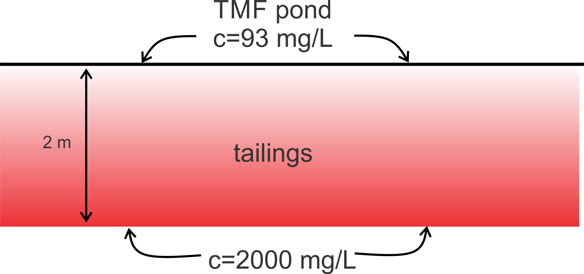
Let’s put the origin \(z=0\) at 2 m depth, so that the pond-sediment interface is at \(z=2~m\). We could also put the origin at the top and set \(z=2~m\) at 2 m into the sediments.
Properties of the problem domain
Here the only property needed to describe steady-state concentration profile is the diffusion coefficient \(D\). For our problem, it’s value was spatially homogeneous \(D=2\times 10^{-10}~m^2/s\).
Boundary conditions
This problem has two prescribed concentration boundary conditions. 1. \(c(0)=2000~mg/L\) at 2 m depth in the sediments (where \(z=0\)). 2. \(c(2)=93~mg/L\) at the pond-sediment interface (where \(z=2~m\)).
Initial conditions
Not required since this is not a time-dependent problem.
Assignment
1 Finding an analytical solution
Let’s see if we can guess the exact solution to the BVP for the TMF diffusion problem. ## Your turn
You are clever, and guess that the concentration profile varies linearly with depth. That is, the function is of the form
\begin{align} c(z) &= az + b\\ \end{align} where \(a\) and \(b\) are some coefficients. What are the values of \(a\) and \(b\) that satisfy the boundary - value problem? Common sense: the solution has to run linearly between the two boundary points. Solve for \(a\) and \(b\) and enter their values in the cell below for autograding, i.e. write two lines of python that set:
a= xxx b=xxx
[5]:
# YOUR CODE HERE
#raise NotImplementedError()
[6]:
# We test your a and b values here
Prove that the analytical “solves” the BVP by:
substituting the analytical expression into the partial differential equation and differentiating (in the same way you proved solutions solved the ODE).
showing that the solution satisfies the boundary conditions. That is, show that \(c(0) = 2000\) and \(c(2) = 93\).
Enter work in the cell below
YOUR ANSWER HERE
What would the profile look like if the diffusion coefficient were 10 times larger? Or 10 times smaller? Explain in the cell below
YOUR ANSWER HERE
If the porosity of the sediments is \(\theta=0.25\), what is the magnitude of the specific diffusive flux \(j\) in units of \(mg/(s\cdot m^2)\). Enter the magnitude of the diffusive flux \(j\) in the cell below for autograding.
Spefically we are expecitng you to write a line in python like:
j=xxx
[7]:
# your answer here

# YOUR CODE HERE
#raise NotImplementedError()
[8]:
# Hidden test here
2 Interpretation
Heat moves by conduction from high temperature to low temperature according to Fourier’s law: \begin{align} \vec{q} = -\kappa\nabla u \label{7pde29}\\ \end{align} where * \(u~\left[\Theta\right]\) is the temperature (typical units of Kelvin)(note that \(\Theta\) is the dimension for temperature) * \(q ~\left[{M \over T^3} \right]\) is the specific heat flux (typical units are Watts per \(m^2\)) * \(\kappa~\left[{M L\over T^3\Theta}\right]\) is the thermal conductivity (typical units are Watts per \(m\) per Kelvin) * \(\nabla u~\left[{\Theta\over L}\right]\) is the temperature gradient (typical units are Kelvin per \(m\)).
1.
Show that the dimensions of the left and right hand of Fourier’s law are the same:
Dimensions of \(q\): \(\left[{M \over T^3} \right]\); Dimensions of \(-\kappa\nabla u\): \(\left[{\text{Your dimensions here}}\right]\)
The partial differential equation that governs heat flow by conduction can be written in vector form \begin{align} &\rho c_p{\partial u\over \partial t} = \nabla \cdot (\kappa \nabla u)\label{7pde30}\\ \end{align} where \(\rho~\left[{M\over L^3}\right]\) is the density of the material through which heat is conducting. This equation is called the heat equation.
2.
What are the dimensions of the specific heat capacity \(c_p\)?
\(c_p~\left[{\text{Your dimensions here}}\right]\)
3.
What is the physical meaning of the the term \(\rho c_p{\partial u\over \partial t}\) in the heat equation \ref{7pde30}?
4.
Write the transient heat equation in non-vector form in two dimensions (\(x\), and \(y\)). Hint: look at diffusion equation examples above.
\begin{align} \text{your equation here} \end{align}