Landsat 8 false color examples

54. Landsat 8 false color examples#

In the Making color composite (“false color”) images notebook we showed how to make a false color composite with Landsat 8 bands 5, 4, 3 mapped to red, blue and green (color infrared)

In this notebook we move that code into a function called make_false_color, and show a Vancouver scene with some different band combinations. We make use of a boolean mask to get a stretched histogram using skimage.exposure that only calculates the stretched histogram for cloud-free pixels over land.

The make_false_color function takes an xarray.Dataset containing an fmask and all the Landsat bands and returns a false color rioxarray.DataArray containing a [3,nrows,ncols] array with the stacked bands.

New functions:

make_dataset function
make_bool_mask function
make_false_color function

54.1. Installation#

Download false_color_examples.ipynb from the week 10 folder
Download the week10 tif files from satdata/landsat/vancouver_2023/week10 and move them to `~/repos/a301/satdata/landsat/week10/

import xarray
import rioxarray
from matplotlib import pyplot as plt
import numpy as np
from skimage import exposure, img_as_ubyte
from IPython.display import Image
from pathlib import Path
from numpy.typing import NDArray

54.2. Understanding Landsat band location#

The figure below shows average reflectances for various surface types. Compare some of thse reflectance values with the landsat band locations in microns

coastal aerosol: 0.44
blue: 0.47
green: 0.55
red: 0.65
near-ir: 0.86
swir1 1.6
swir2: 2.2

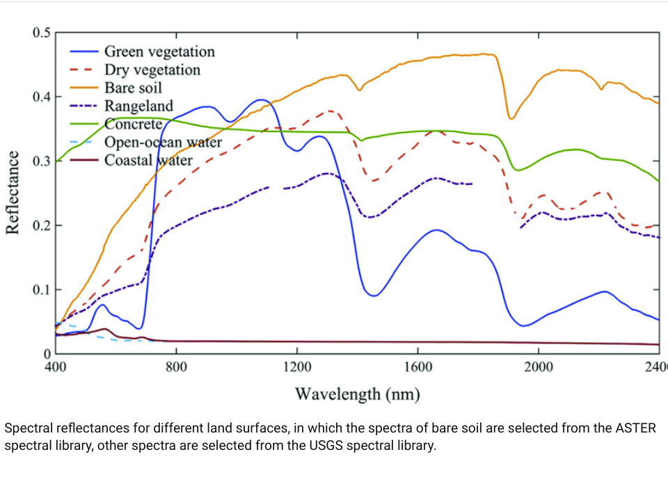
../../_images/hou_reflectance.png — Fig. 54.1 Reflectance spectra#

54.3. Landsat bands by surface type#

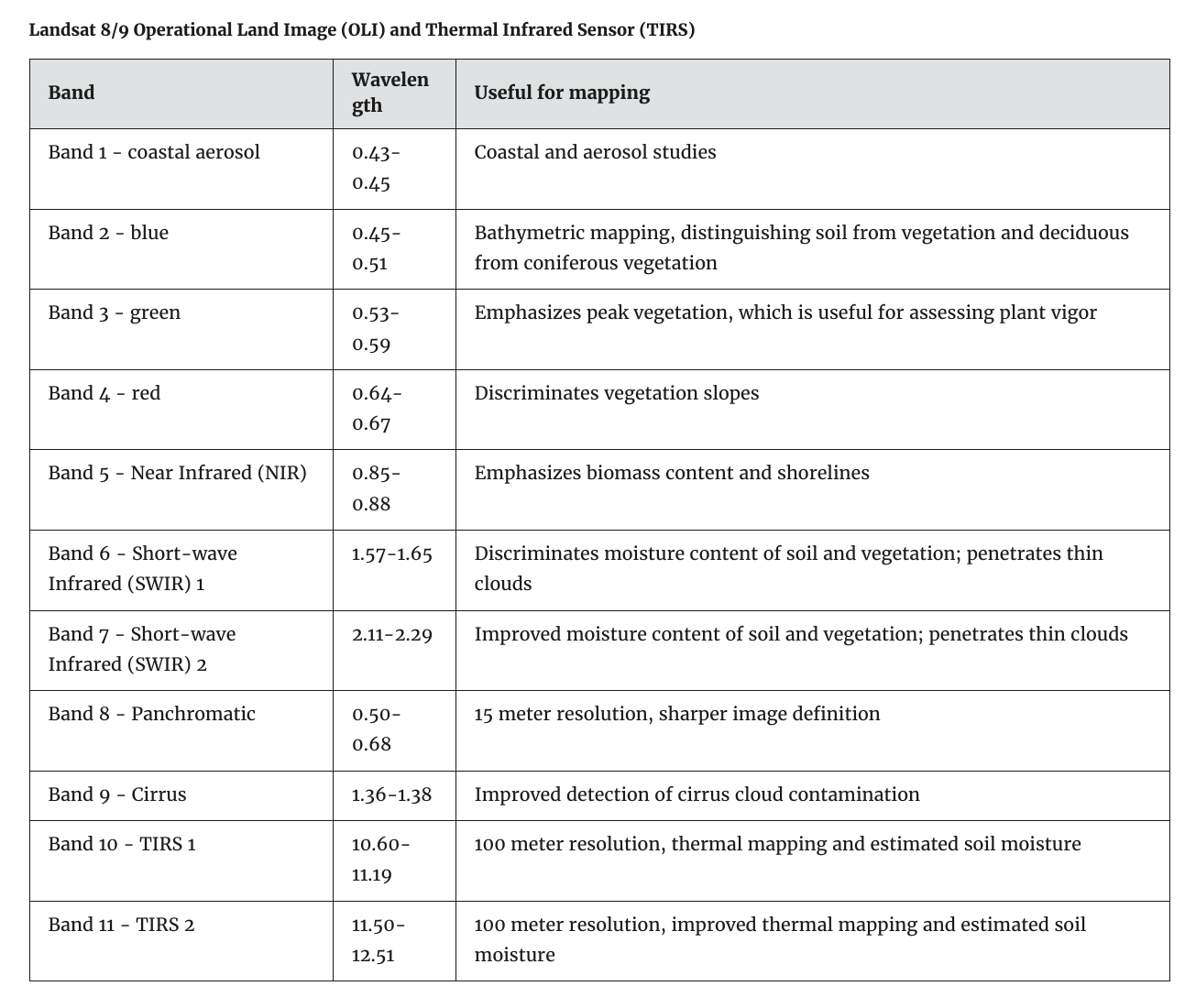
../../_images/landsat8_bands.png — Fig. 54.2 Landsat 8 band wavelengths#

54.4. Landsat false color combinations#

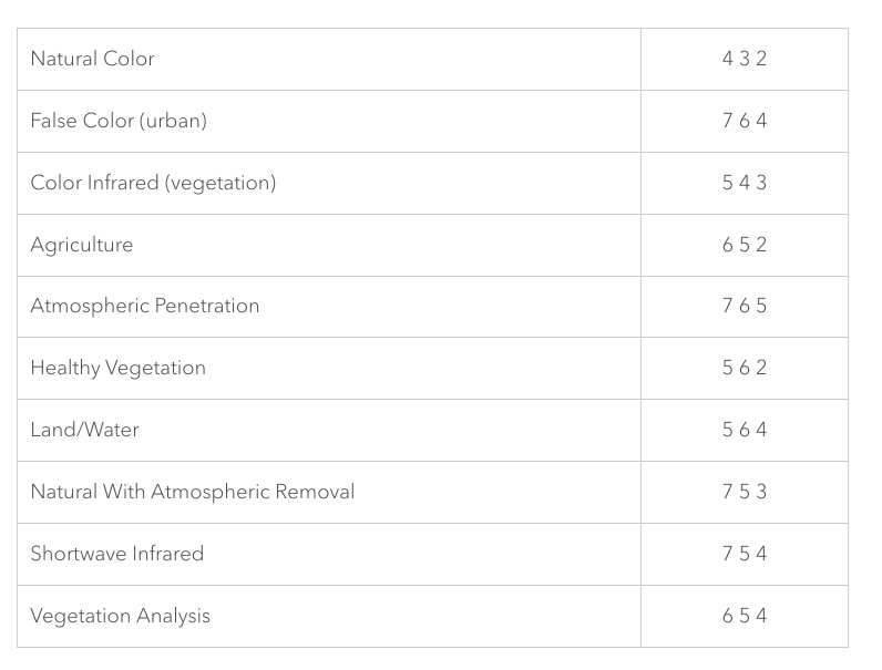
54.4.1. Specific examples#

see this website for images that demonstrate the combinations
see this goes2go demo for mulitple GOES band combinations

54.5. False color bands for Vancouver#

bands={'B01':'Coastal_Aerosol',
        'B02':'Blue',
        'B03':'Green',
        'B04':'Red',
        'B05':'NIR',
        'B06':'SWIR1',
        'B07':'SWIR2',
        'B09':'Cirrus',
        'B10':'TIRS1',
        'B11':'TIRS2',
        'fmask':'fmask'}

54.5.1. Read all bands into a dictionary#

Use the bands dictionary to identify the band by its name (Blue, Green, etc) and store it in scene_dict. Masking fmask would convert it from 8 bit to float, so we need to special-case the fmask file.

data_dir = Path().home() / 'repos/a301/satdata/landsat'
all_tifs = list(data_dir.glob('**/week10*clipped_*.tif'))
scene_dict = {}
for key,bandname in bands.items():
    band_tif = None
    for the_tif in all_tifs:
        if str(the_tif).find(bandname) > -1:
            print(f"reading {key}:{the_tif}")
            if key == 'fmask':
                scene_dict[key] = rioxarray.open_rasterio(the_tif)
            else:
                scene_dict[key] = rioxarray.open_rasterio(the_tif, mask_and_scale=True)
            continue
   
    

reading B01:/Users/phil/repos/a301/satdata/landsat/vancouver_2023/week10/week10_clipped_Coastal_Aerosol.tif
reading B02:/Users/phil/repos/a301/satdata/landsat/vancouver_2023/week10/week10_clipped_Blue.tif
reading B03:/Users/phil/repos/a301/satdata/landsat/vancouver_2023/week10/week10_clipped_Green.tif
reading B04:/Users/phil/repos/a301/satdata/landsat/vancouver_2023/week10/week10_clipped_Red.tif
reading B05:/Users/phil/repos/a301/satdata/landsat/vancouver_2023/week10/week10_clipped_NIR.tif
reading B06:/Users/phil/repos/a301/satdata/landsat/vancouver_2023/week10/week10_clipped_SWIR1.tif
reading B07:/Users/phil/repos/a301/satdata/landsat/vancouver_2023/week10/week10_clipped_SWIR2.tif
reading B09:/Users/phil/repos/a301/satdata/landsat/vancouver_2023/week10/week10_clipped_Cirrus.tif
reading B10:/Users/phil/repos/a301/satdata/landsat/vancouver_2023/week10/week10_clipped_TIRS1.tif
reading B11:/Users/phil/repos/a301/satdata/landsat/vancouver_2023/week10/week10_clipped_TIRS2.tif
reading fmask:/Users/phil/repos/a301/satdata/landsat/vancouver_2023/week10/week10_clipped_fmask.tif

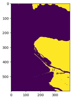
54.5.3. make_bool_mask function#

def make_bool_mask(
      da_fmask:xarray.DataArray
     ) -> NDArray[np.uint8]:
    """'
    turn a Landsat fmask into a boolean 1/0 array where
    cloud-free land pixels are 1 and all other pixels are 0
    For use by skimage.exposure.equalize_hist

    Parameters
    ----------

    da_fmask: the fmask DataArray

    Returns: bool_mask with the same shape
    """
    scene_mask = da_fmask.data
    mask_select =  0b00100011  #find water (bit 5), cloud (bit 1) , cirrus (bit 0)
    ref_mask = np.zeros_like(scene_mask)
    ref_mask[...] = mask_select
    masked_values = np.bitwise_and(scene_mask,ref_mask)
    masked_values[masked_values>0]=1  #cloud or water
    masked_values[masked_values==0]=0 #rest of scene
    #
    # now invert this, writing 1 for 0 and 0 for 1
    # use 9 as a placeholder value
    bool_mask = masked_values[...]
    bool_mask[masked_values==1] = 9
    bool_mask[masked_values==0] = 1
    bool_mask[masked_values==9] = 0
    return bool_mask
    
    
    
    

bool_image = make_bool_mask(scene_dict['fmask'])
plt.imshow(bool_image.squeeze())

<matplotlib.image.AxesImage at 0x127394ad0>

../../_images/2bbfd646cad5adeef4de476e9fa49e6f2203a25bf1faf280be1c8825cec92850.png

54.5.4. make_false_color function#

def make_false_color(
        the_ds: xarray.Dataset,
        band_names: list[str]) -> xarray.DataArray:
    """
    given a landsat dataset created with at least an fmask and 3 bands,
    return a histogram-equalized false color image with rgb mapped
    to the bands in the order they appear in the list band_names

    example usage:

    landsat_654 = make_false_color(the_ds,['B06','B05','B04'])

    Parameters
    ----------

    the_ds:
       created by make_dataset -- must contain at least 3 bands and Fmask
    band_names: 
       list of strings with the names of the bands to be mapped to red, green and blue

    Returns
    -------

    false_color: rioxarray with shape [3,nrows,ncols] that can be converted to png
    """
    the_ds = the_ds.squeeze()
    rgb_names = ["band_red", "band_green", "band_blue"]
    #
    # dictionary to hold the 3 rgb bands
    #
    scene_dict = dict()
    for the_rgb, the_band in zip(rgb_names, band_names):
        # print(f"{the_rgb=}, {the_band=}")
        scene_dict[the_rgb] = the_ds[the_band]
    crs = the_ds.rio.crs
    transform = the_ds.rio.transform()
    fmask = the_ds["fmask"].data
    bool_mask = make_bool_mask(fmask)
    #
    # histogram equalize the 3 bands
    #
    for key, image in scene_dict.items():
        scene_dict[key] = exposure.equalize_hist(image.data, mask=bool_mask)
    nrows, ncols = bool_mask.shape
    band_values = np.empty([3, nrows, ncols], dtype=np.uint8)
    #
    # convert to 0-255
    #
    for index, key in enumerate(rgb_names):
        stretched = scene_dict[key]
        band_values[index, :, :] = img_as_ubyte(stretched)
    #
    # only keep a subset of the attributes
    #
    keep_attrs = ["cloud_cover", "date", "day", "target_lat", "target_lon"]
    all_attrs = the_ds.attrs
    attr_dict = {key: value for key, value in all_attrs.items() if key in keep_attrs}
    attr_dict["history"] = "written by make_false_color"
    attr_dict["landsat_rgb_bands"] = band_names
    band_nums = [int(item[-1]) for item in band_names]
    coords = {"band": band_nums, "y": the_ds["y"], "x": the_ds["x"]}
    dims = ["band", "y", "x"]
    # print(f"{dims=}")
    # print(f"{band_values.shape=}")
    false_color = xarray.DataArray(
        band_values, coords=coords, dims=dims, attrs=attr_dict
    )
    false_color.rio.write_crs(crs, inplace=True)
    false_color.rio.write_transform(transform, inplace=True)
    return false_color

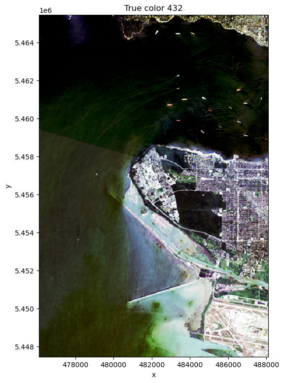
54.6. True color (red, green, blue)#

true_color = make_false_color(ds_allbands, band_names=["B04","B03","B02"])
fig1, ax1 = plt.subplots(1,1,figsize=(6,9))
true_color.plot.imshow(ax=ax1);
ax1.set(title="True color 432");

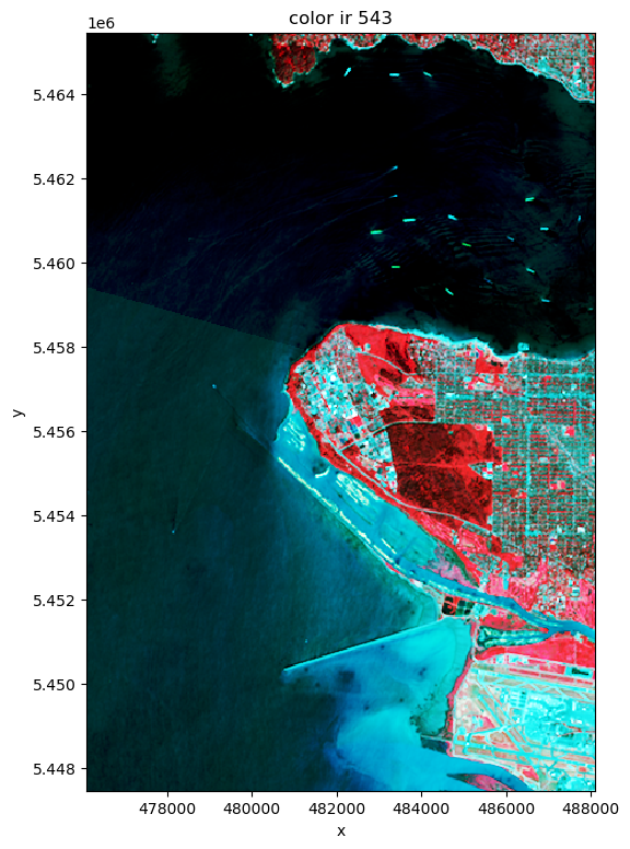
../../_images/a679d3276f9c16e91a0fe263435b1100331fe8107151ac2d80cc8f65865a54d7.png

54.7. Color infrared: near-ir, red, green#

Add the 5-4 red edge for vegetation, plus green (also vegetation). See band543 detail

color_ir = make_false_color(ds_allbands, band_names=["B05","B04","B03"])
fig2, ax2 = plt.subplots(1,1,figsize=(6,9))
color_ir.plot.imshow(ax=ax2);
ax2.set(title="color ir 543");

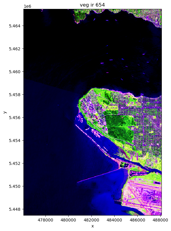
../../_images/271b48269f0da7afe5a72f1b381dd41bdb299346074778167e0487756a9c57f8.png

54.8. Vegetation swir-1, near-ir, red#

Add swir-1 for moisture content, keep the 5-4 red edge. Less contrast for turbid/fresh water. See band654 detail

veg_ir = make_false_color(ds_allbands, band_names=["B06","B05","B04"])
fig3, ax3 = plt.subplots(1,1,figsize=(6,9))
veg_ir.plot.imshow(ax=ax3);
ax3.set(title="veg ir 654");

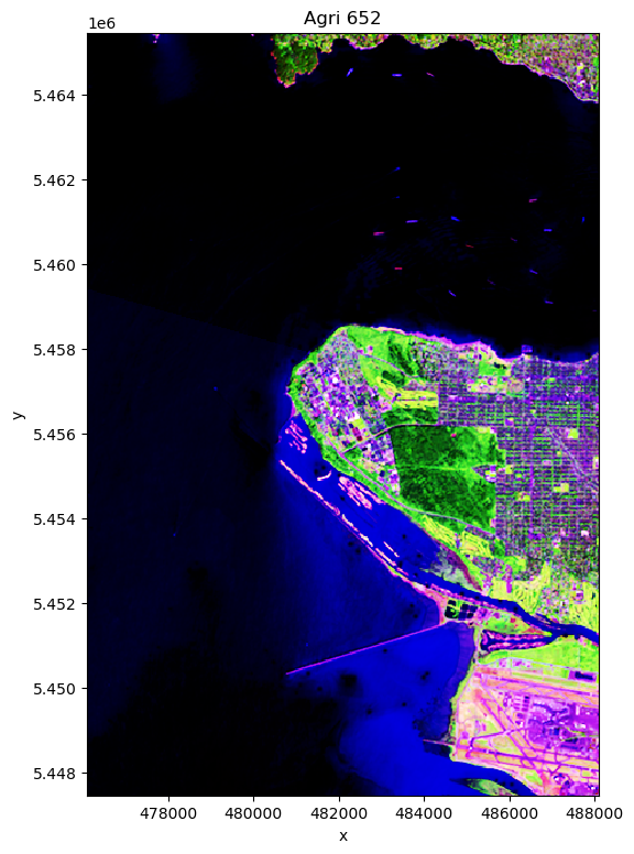
../../_images/51e0cb5e2444e95cd2c14cf3c313aa5fa033aa6f80e80f542889d7d932a7baec.png

54.9. Agriculture swir-1, near-ir, blue#

Swap out red for blue. See band652 detail

agri = make_false_color(ds_allbands, band_names=["B06","B05","B02"])
fig4, ax4 = plt.subplots(1,1,figsize=(6,9))
agri.plot.imshow(ax=ax4);
ax4.set(title="Agri 652");

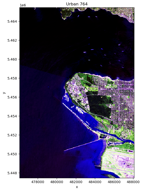
../../_images/dbf730836a3d300c9fd01db61e1a489fdde92e82a6e5e9e96f50e011395f0156.png

54.10. Urban swir-2, swir-1, red#

concrete and bare soil have approximately constant reflectivities between 1.6 and 2.2 microns, while vegetation reflects more in swir-1 than swir-2. This combination distinguishes between types of urban development. Less contrast for turbid/fresh water. See: band764 detail

urban = make_false_color(ds_allbands, band_names=["B07","B06","B04"])
fig5, ax5 = plt.subplots(1,1,figsize=(6,9))
urban.plot.imshow(ax=ax5);
ax5.set(title="Urban 764");

../../_images/accacacd09935f70cd5d4a486bd5ede7d65115a70c7fb4cf7118d5db371887e5.png