51. Calculating the diffuse flux: python code

import matplotlib
import matplotlib.pyplot as plt
import numpy as np
from scipy.special import expn

In the Integrating the Schwartzchild equation notes I claimed that the following approximation was a good one:

(51.1)\[ \hat{t}_f = 2 \int_0^1 \mu \exp \left (- \frac{\tau }{\mu} \right ) d\mu \approx \exp \left (-1.66 \tau \right ) \]

As I mentioned, we can’t calculate this integral analytically, but it’s important enough that it has its own special function in python: scipy.special.expn

Below we use this function to compare the approximate version np.exp(-1.66*tau) with a brute force integration and the expn more exact answer.

51.1. Change of variables

First we need to show that (51.1) the is actually the third exponential integral. This requires doing a change of variables:

\[u = \mu^{-1}\]

Use this substitutiion to show that we can rewrite (51.1) as:

\[ \hat{t}_f = 2 \int_1^\infty \frac{\exp(-u \tau)}{u^3} du \]

which is available from scipy as expn(3.0, tau)

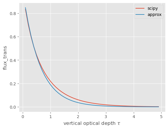
The next cell shows the approximate and exact values vs the vertical (straightup) optical depth \(\tau\)

"""
   plot 2*scipy.special.expn(3,the_tau))
   this is the accurate version of the flux transmission function
   defined above
"""

matplotlib.style.use("ggplot")
tau = np.arange(0.1, 5, 0.1)
flux_trans = 2 * expn(3.0, tau)
fig, ax = plt.subplots(1, 1)
ax.plot(tau, flux_trans, label="scipy")
ax.plot(tau, np.exp(-1.66 * tau), label="approx")
ax.legend()
ax.set(ylabel="flux_trans", xlabel=r"vertical optical depth $\tau$")

[Text(0, 0.5, 'flux_trans'), Text(0.5, 0, 'vertical optical depth $\\tau$')]

51.2. Brute force approx

What if scipy hadn’t provided the expn function? We can also do a brute-force approximation using rectangle area

def trans_fun(tau,mu):
    """
    equation 1 above
    """
    output = 2*mu*np.exp(-tau/mu)
    return output

def do_int(tau,mu_vec):
    """
    rectangular integration
    """
    
    trans_vec=np.empty_like(mu_vec)
    
    for index, the_mu in enumerate(mu_vec):
        trans_vec[index]=trans_fun(tau,the_mu)
    dmu=np.diff(mu_vec)
    mid_trans = (trans_vec[1:] + trans_vec[:-1])/2.
    return np.sum(mid_trans*dmu)       
    

mu_vec = np.linspace(0.01,1,150)
tau_vec=np.arange(0.1,5,0.1)
flux_trans = np.empty_like(tau_vec)
for index,tau in enumerate(tau_vec):
    flux_trans[index] = do_int(tau,mu_vec)
    
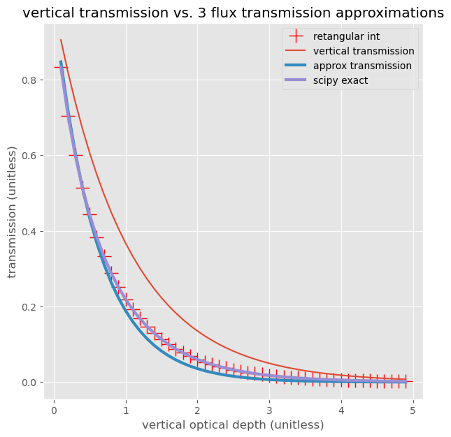
fig, ax = plt.subplots(1,1,figsize=(7,7))
ax.plot(tau_vec,flux_trans,'r+',markersize=15,label="retangular int");
ax.set_xlabel('vertical optical depth (unitless)')
ax.set_ylabel('transmission (unitless)')
ax.plot(tau_vec,np.exp(-tau_vec),label='vertical transmission')
ax.plot(tau_vec,np.exp(-1.666*tau_vec),label='approx transmission',lw=3)
flux_trans = 2 * expn(3.0, tau_vec)
ax.plot(tau_vec,flux_trans,label='scipy exact',lw=3)
ax.set_title("vertical transmission vs. 3 flux transmission approximations")

ax.legend();