41. Using fmask to mask water pixels

41.1. Intoduction

• Download the fmask.ipynb notebook from week7 in our gdrive folder

• Download the folder downloads/vancouver/week7 containing the clipped tif files produced by v0.2 of Clipping multiple bands– v0.3 and a new fmask file ~/repos/a301/satdata/landsat/vancouver

In Making color composite (“false color”) images we created false color images using 3 bands. One problem with those images is that half of the scene was water, which we aren’t particularly interested in. In this notebook we use a mask file downloaded from NASA (HLS.L30.T10UDV.2015165T190019.v2.0.Fmask.tif) using Landsat 1: Dowloading Landsat and Sentinel data from NASA to remove all the water pixels. It cleans up the joint histograms significantly.

41.2. Read in the clipped image

Copy some code from Making color composite (“false color”) images

import xarray
import rioxarray
from pathlib import Path
from matplotlib import pyplot as plt
import numpy as np
import seaborn as sns
from skimage import exposure, img_as_ubyte
from IPython.display import Image
from a301_lib import make_pal

41.2.1. Add the fmask to the list

data_dir = Path().home() / 'repos/a301/satdata/landsat/vancouver'
blue = list(data_dir.glob('**/*Blue*tif'))[0]
red = list(data_dir.glob('**/*Red*tif'))[0]
green = list(data_dir.glob('**/*Green*tif'))[0]
nir =  list(data_dir.glob('**/*NIR*tif'))[0]
fmask =  list(data_dir.glob('**/*Fmask*tif'))[0]
band_dict = dict(zip(('red','green','nir','blue','fmask'),(red,green,nir,blue,fmask)))

xarray_dict={}
for key,filename in band_dict.items():
    print(key)
    xarray_dict[key] = rioxarray.open_rasterio(filename,mask_and_scale=True);
    xarray_dict[key] = xarray_dict[key].squeeze()

red
green
nir
blue
fmask

41.3. Clip fmask to the same bounding box

Copy some code from Clipping multiple bands– v0.3

clipped_tif = xarray_dict['blue']
clipped_transform = clipped_tif.rio.transform()
nrows, ncols = clipped_tif.shape
ul_x, ul_y = clipped_transform * (0, 0)
lr_x, lr_y = clipped_transform * (ncols, nrows)
bounding_box = (ul_x, lr_y, lr_x, ul_y)
print(f"{bounding_box=}")
fmask = xarray_dict['fmask'].rio.clip_box(*bounding_box)

bounding_box=(476100.0, 5447460.0, 488100.0, 5465460.0)

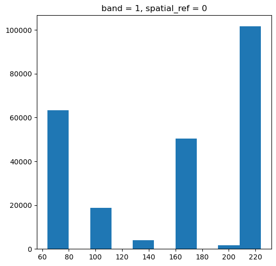
41.3.1. fmask data

This scene has 6 unique fmask values

fmask.plot.hist(figsize=(6,6));

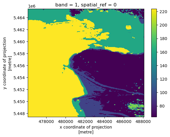
41.3.2. fmask image

fmask.plot.imshow();

41.4. decoding fmask values

So what is the meaning of these six numbers? The values are given in the hls landsat user guide on page 17

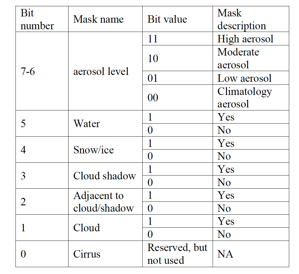
Fig. 41.1 hls landsat fmask values

The full scene before clipping acually has 35 values:

len(np.unique(xarray_dict['fmask'].data))

35

Here’s how to list the individual bit order for each number in the mask. We need to convert the floating point values to unsigned, 8 bit integers (uint8) and then unpack the 8 bits using the numpy function unpackbits

var = xarray_dict['fmask'].data
var = fmask.data
vals = np.unique(var)
vals = vals.astype('uint8')
for item in vals:
    print(f"{item:03d}",np.unpackbits(item))

064 [0 1 0 0 0 0 0 0]
096 [0 1 1 0 0 0 0 0]
128 [1 0 0 0 0 0 0 0]
160 [1 0 1 0 0 0 0 0]
192 [1 1 0 0 0 0 0 0]
224 [1 1 1 0 0 0 0 0]

Comparing with the table, you should recognize that 96, 160, and 224 all have their bit 5 (counting from the right) set to 1, indicating water. The difference between the three is whether they have clean air (01 in bits 6,7), moderate aerosols (10) or high aerosols (11).

41.5. finding all water pixels

How do we find the water pixels for the clipped scene? We want to find all pixels in the mask with their bit 5 set to 1. We can do that by creating a mask with only the bit 5 set to 1, then doing a bitwise_and with the masked values. That will turn the water pixels into decimal 32 (2**5), and all other pixels into 0, because only (1 and 1) is 1, and all other bit postions with and to zero.

bit5_on = 0b00100000
#
# construct an array of the right shape filled with
# the water bit
#
a_array = np.full(fmask.data.shape,bit5_on)
#
# turn the fmask values into unsigned bytes
#
var_bytes = fmask.data.astype('uint8')
#
# do the bitwise_and to get a mask
#
water_mask = np.bitwise_and(var_bytes,a_array)

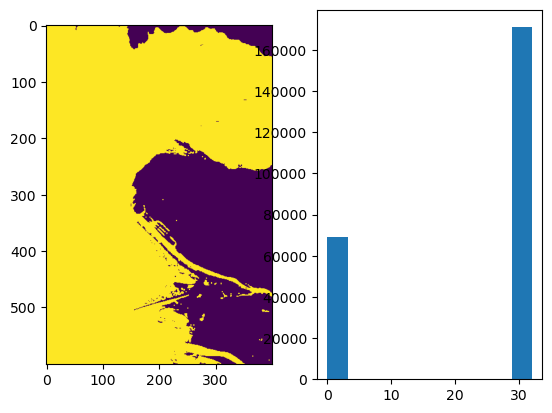
41.5.1. plot the water_mask

As expected, water=32, everything else is 0.

fig, (ax1,ax2) = plt.subplots(1,2)
ax1.imshow(water_mask)
ax2.hist(water_mask.flat);

41.5.2. Inverting the water mask

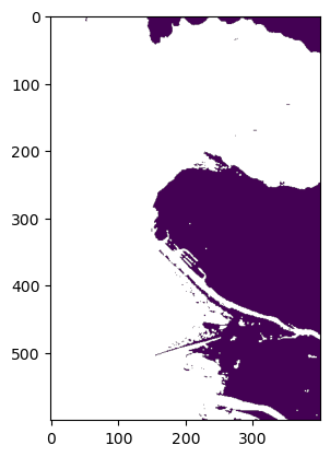
Now that we know where the water is, we want to assign all those pixels as np.nan, and all land pixels as 1. We can do this using np.where. The next cell assigns all the land pixels the value 1, and all other pixels the value np.nan

land_mask = np.where(water_mask == 0,1,np.nan)

plt.imshow(land_mask);

41.6. Using the mask

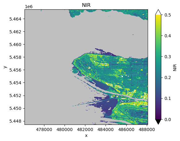
Now that we have the land_mask, we multiply the data by the mask to remove water pixels, like this:

varname = 'nir'
xarray_dict[varname].data = xarray_dict[varname].data*land_mask

vmin = 0.0
vmax = 0.5
pal_dict = make_pal(vmin=vmin,vmax=vmax)
fig, ax = plt.subplots(1,1)
var = 'nir'
xarray_dict[var].plot.imshow(ax=ax,
                    norm = pal_dict['norm'],
                    cmap = pal_dict['cmap'],
                    extend = "both")
ax.set(title=f"{xarray_dict[var].long_name}");

41.6.1. Mask the remaining bands

Do this to every band except fmask

for key,array in xarray_dict.items():
    if key=='fmask':
        continue
    array.data = array.data*land_mask

41.6.2. Give the bands shorter names

Makes it easier to type

b2, b3, b4, b5 = (xarray_dict['blue'],xarray_dict['green'], 
                   xarray_dict['red'], xarray_dict['nir'])

41.7. Plotting joint histograms

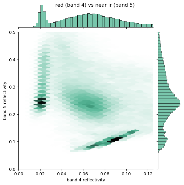
Compare the masked joint histograms with the ones we found in Plotting joint histograms. They are much cleaner.

fig = sns.jointplot(
    x=b3.data.ravel(),
    y=b4.data.ravel(),
    xlim=(0, 0.125),
    ylim=(0.0, 0.125),
    kind="hex",
    color="#4CB391",
    gridsize=100
)
fig.fig.suptitle("green (band 3) vs red (band 4)");
axes = fig.fig.get_axes()
axes[0].set(xlabel = "band 3 reflectivity",
            ylabel = "band 4 reflectivity");

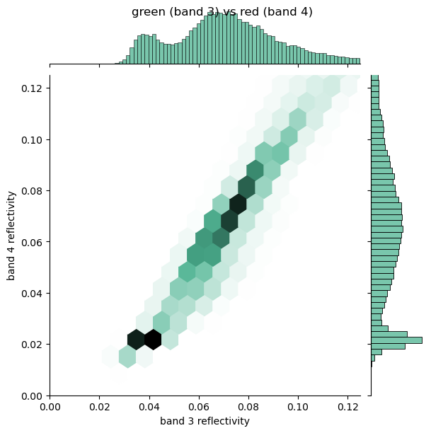
fig = sns.jointplot(
    x=b4.data.ravel(),
    y=b5.data.ravel(),
    kind="hex",
    xlim=(0, 0.125),
    ylim=(0.0, 0.5),
    color="#4CB391",
    gridsize=100
)
fig.fig.suptitle("red (band 4) vs near ir (band 5)");
axes = fig.fig.get_axes()
axes[0].set(xlabel = "band 4 reflectivity",
            ylabel = "band 5 reflectivity");

41.8. Caveat

Histogram equalization won’t work with masked scenes, since exposure.equalize_hist won’t work with nans. That’s not a real problem though, because equalization if more about getting a qualitative, instead of a quantitative, impression.

41.9. Assignment 5 part 2: make a cloud mask function

Due next Friday

Write a function that takes an image and its fmask and returns a new image with all cloudy pixels set to np.nan. Make a notebook that uses this function to plot a partly cloudy scene.