17. Mapping the landsat scene

In this notebook we read in the large (3660 x 3660 pixel) landsat band5 file we downloaded in the Landsat 1: Dowloading Landsat and Sentinel data from NASA notebook. In this notebook we use cartopy to plot the image along with the coastline on a georeferenced map.

• Download map_landsat.ipynb from the week3 folder

17.1. bugfix Jan 20, 2025

Now working with change at Bug: don’t hardcode the dimensions

17.2. Open the band 5 image and read it in to a DataArray

import numpy
from pathlib  import Path
from matplotlib import pyplot as plt
import numpy as np
from copy import copy
import rioxarray
from cartopy import crs as ccrs
import cartopy

data_dir = Path().home() / 'repos/a301/satdata/landsat'
band_name = 5
data_dir.mkdir(exist_ok=True, parents=True)
disk_file = data_dir / f"hls_landsat8_{band_name}.tif"
has_file = disk_file.exists()

if not has_file:
    raise IOError(f"can't find {disk_file}, rerun with the week2 get_landsat_scene notebook") 
hls_band5 = rioxarray.open_rasterio(disk_file,masked=True)

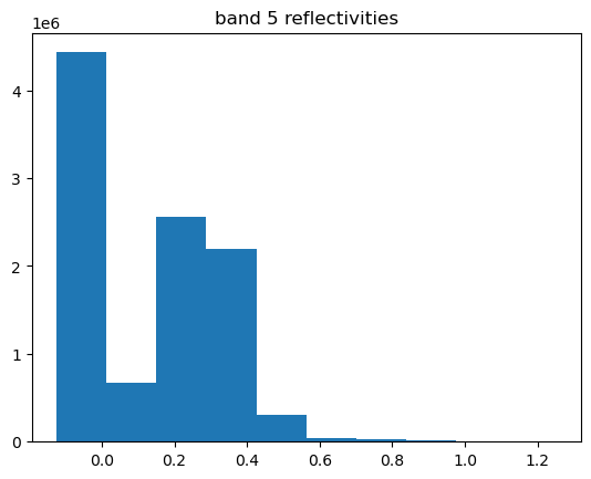
17.3. Scale and histogram the scene using the scale_factor

The data are stored as integer values, we need to divide by 10,000 to convert to surface reflectivities. Make sure the band 5 values look reasonable

hls_band5.scale_factor

0.0001

scaled_band = hls_band5*hls_band5.scale_factor
scaled_band=scaled_band.squeeze()

fig, ax = plt.subplots(1,1)
scaled_band.plot.hist(ax = ax)
ax.set(title="band 5 reflectivities");

17.4. Put the image on a cartopy map

To put our raster image on a longitude/latitude map we need to be able to go back and forth between three different pixel coordinates

1. We need to translate between longitude/latitude and the (x,y) coordinates in our chosen map projection. This the job of the coordinate reference system (CRS) and the python projection module.

2. We need to translate between the (x,y) coordinate system and the row,column numbers of our raster. This is the job of the affine transform

17.4.1. Understanding the affine transform

For our gridded image, we know the coordinates of the upper left corner (ULX, ULY), the size of each pixel \(\Delta x, \Delta y\) (30 meters wide and high), and the number of rows and columns (3660 x 3660). Suppose we want the (x,y) coordinates of the upper left corner of the pixel at row=100,col=300? Convince yourself that this is given by:

\[\begin{split} x &= ULX + col \times \Delta x \\ y &= ULY - row \times \Delta y \end{split}\]

where the negative sign means that the rows increase from top to bottom in the raster. That information is stored in the geotiff as a \(2 \times 3\) matrix called the affine transform.

Here is how you read the transform for the geotiff in rioxarray:

17.4.2. Get the transform from the geotif

print(f"{hls_band5.ULX=} m\n{hls_band5.ULY=} m\n{hls_band5.SPATIAL_RESOLUTION=} m")
the_transform = hls_band5.rio.transform()
print(f"\nthe affine transform is: \n{the_transform}")

hls_band5.ULX=399960 m
hls_band5.ULY=5500020 m
hls_band5.SPATIAL_RESOLUTION=30 m

the affine transform is: 
| 30.00, 0.00, 399960.00|
| 0.00,-30.00, 5500020.00|
| 0.00, 0.00, 1.00|

A good explanation for what all the other items in the matrix are is given in Matthew Perry’s blog post. As he shows, using the transform we can get (x,y) by using the definition of the * operation created by the transform object.

17.4.3. Using the transform to convert (row,col) to (x,y)

Get the (x,y) of the upper left corner using *

x_ul, y_ul = the_transform*(0,0)
x_ul, y_ul

(399960.0, 5500020.0)

get the (x,y) of the lower right corner

17.4.4. Bug: don’t hardcode the dimensions

x_lr, y_lr = the_transform*(3661,3361)

that should be the number of columns, number of rows – lesson learned: avoid hard coding numbers wenever possible

nrows, ncols = scaled_band.shape
x_lr, y_lr = the_transform*(ncols, nrows)
x_lr, y_lr

(509760.0, 5390220.0)

Note that we need to add 1 to (nrows,ncols) because we want the lower right edge of the bottom pixel, not its upper left corner.

17.5. Setting up the cartopy map

Now set up a map with the correct extent in the x and y directions and correct crs. Recall how we did this in Mapping Vancouver with cartopy

First get the map projection. Unforunately cartopy requires an epsg code to create the crs, and the geotiff crs provides a name (UTM Zone 10) but not a code. By googling you can see that the code epsg:32610. A rather hacky way to make that jump is to convert geotiff code to Well Known Text (WKT) and create a pyproj CRS object, which knows how to output its most likely epsg code. Here are the two steps:

17.5.1. 1. dump the crs into a wkt string

from pyproj.crs import CRS
utm10 = hls_band5.rio.crs.to_wkt()
utm10

'PROJCS["UTM Zone 10, Northern Hemisphere",GEOGCS["Unknown datum based upon the WGS 84 ellipsoid",DATUM["Not specified (based on WGS 84 spheroid)",SPHEROID["WGS 84",6378137,298.257223563,AUTHORITY["EPSG","7030"]]],PRIMEM["Greenwich",0],UNIT["degree",0.0174532925199433,AUTHORITY["EPSG","9122"]]],PROJECTION["Transverse_Mercator"],PARAMETER["latitude_of_origin",0],PARAMETER["central_meridian",-123],PARAMETER["scale_factor",0.9996],PARAMETER["false_easting",500000],PARAMETER["false_northing",0],UNIT["metre",1,AUTHORITY["EPSG","9001"]],AXIS["Easting",EAST],AXIS["Northing",NORTH]]'

17.5.2. 2. make a cartopy crs object from the wkt string using the pyproj crs

proj_crs = CRS.from_wkt(utm10)
pyproj_epsg = proj_crs.to_epsg(min_confidence=60)
print(f"{pyproj_epsg=}")
cartopy_crs = ccrs.epsg(pyproj_epsg)
cartopy_crs

pyproj_epsg=32610

<cartopy._epsg._EPSGProjection object at 0x141649e80>

cartopy_crs.to_epsg()

32610

Borrow code from Mapping Vancouver with cartopy for the palette

pal = copy(plt.get_cmap("viridis"))
pal.set_bad("0.75")  # color 75% grey np.nan cells
pal.set_over("w")  # color cells > vmax red
pal.set_under("k")  # color cells < vmin black
vmin = 0.0  #anything under this is colored black
vmax = 0.8  #anything over this is colored white
from matplotlib.colors import Normalize
the_norm = Normalize(vmin=vmin, vmax=vmax, clip=False)

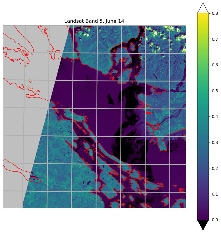
17.6. Plot the image and map together

Looks like the cartopy coastlines and the landsat image are offset a little in the north-south direction, needs some debugging. Note the alpha=0.4 parameter in the imshow call – that makes the image semi-transparent so we can see the coastlines. Note that, unfortunately, cartopy has decided to call the crs the transform.

scaled_band.shape

(3660, 3660)

fig, ax = plt.subplots(1, 1, figsize=(10, 10), subplot_kw={"projection": cartopy_crs})
the_extent=[x_ul, x_lr,y_lr,y_ul]
ax.set_extent(the_extent,cartopy_crs)
ax.gridlines(linewidth=2)
ax.add_feature(cartopy.feature.GSHHSFeature(scale="auto", levels=[1, 2, 3],edgecolor='red'))
cs = ax.imshow(
    scaled_band,
    transform=cartopy_crs,
    extent=the_extent,
    origin="upper",
    alpha=1,
    cmap=pal,
    norm=the_norm
)
ax.set(title="Landsat Band 5, June 14")
fig.colorbar(cs, extend="both");

17.7. Summary

1. Geotiffs carry two metadata items needed for mapping:

   • The affine transform, which relates (row, col) on the raster to (x, y) on the map

   • The coordinate reference system, which relates (x, y) on the map to (lat, lon) on the sphere

2. In cartopy, the crs is called the transform (unfortunate confusion with the affine transform), and the (x,y) coordinates of the left, right, bottom, top of the image is called the extent

3. To put an image on a map, create an axis with the map projection, set the extent of the map, add coastlines, then add the image using imshow with the crs and extent you’ve used to create the axis.

4. There is a standard set of codes for thousands of different crs, called the epsg registry. All modern gis software is able to work with these codes, although not necessarily elegantly.