6. A301 midterm solutions

Name (Last, First):

Student Number:

Instructions: Answer all questions, clearly labeling each answer, showing all your work on the exam booklet.

For partial credit: If you’re stuck on one part of a multipart question and need to move on, you can invent a reasonable set of numbers so that you can answer subsequent questions for full credit. Just be very clear in explaining what you’re doing.

Closed book, equation sheet provided, calculators ok

6.1. Q1) (12)

A satellite orbiting at an altitude of 36000 km observes the surface in the \(CO_2\) absorption band with a wavelength range of 14 μm  \(< λ < 16\) μm.

6.1.1. Q1a) (4 points)

The atmosphere is 20 km thick, and has a density scale height of \(H_\rho\) = 9 km and a surface air density of \(\rho_{air}\) = 1.1 \(kg\,m^{-3}\). The \(CO_2\) mass absorption coefficient is \(k_λ\) = 0.15 \(m^2\,kg^{-1}\) at λ = 15 μm and its mixing ratio is \(4 \times 10^{−4}\,kg\,kg^{-1}\). Find the:

• the atmosphere’s vertical optical thickness \(τ_λ\) in the \(CO_2\) band

• the atmosphere’s transmittance \(t_\lambda\) in the \(CO_2\) band

for a pixel directly beneath the satellite.

6.1.1.1. Q1a answer

\[\begin{split} \rho(z) &= \rho_0 r_{mix} \exp( -z/H_\rho) \\ \tau_T &= \int_0^{20} \rho_0 r_{mix} \exp(-z/H) k_\lambda dz = - H \rho_0 r_{mix} k_\lambda (\exp(-20/9)-1)\\ \tau_T &= 9000 \times 4 \times 10^{-4} *0.15 * (1 - 0.108) = 0.53\\ t_T &= \exp(-\tau_T) = 0.589 \end{split}\]

6.1.2.

Q1b (4 points)

If the surface is a blackbody with a temperature of 290 K, and the atmosphere has an constant temperature of 270 K, find the

• monochromatic radiance observed by the satellite at 15 μm in (\(W\,m^{-2}\,\mu m^{-1}\,sr^{-1}\))

• the brightness temperature of the pixel in Kelvins for that radiance

6.1.2.1. Q1b answer

From the Planck diagram, at \(\lambda=15\ \mu m\) I get:

• \(L_0 \approx 6\ W\,m^{-2}\,\mu m^{-1}\,sr^{-1}\)

• \(B_\lambda \approx 4.6\ W\,m^{-2}\,\mu m^{-1}\,sr^{-1}\)

Use equation (28) from the equation sheet, assume looking straight down so \(\mu = 1\):

\[ L_\lambda(\tau/\mu)= B_\lambda(T_{skin}) \hat{t}_{tot} + (1 - \exp(-\tau/\mu) )B_\lambda(T) \]

\[L_\uparrow(\tau_T) = 6 \times 0.589 + (1 - 0.589) \times 4.6 = 5.41\ W\,m^{-2}\,\mu m^{-1}\,sr^{-1}\]

From the Planck diagram 5.41 \(W\,m^{-2}\,\mu m^{-1}\,sr^{-1}\) at 15 \(\mu m\) is a brightness temperature of about 282 K.

6.1.3. Q1c (4 points)

• Given a pixel size \(10\ km^2\), find:

  • the imager field of view in steradians

  • the flux, in \(W\,m^{-2}\) at the satellite for the wavelength range between 14-16 \(\mu m\)

6.1.3.1. Q1C answer

\(\Delta \omega\) = \(\frac{area}{R^2}\) = \(\frac{10}{36000^2}\) = \(7.7 \times 10^{-9}\ sr\)

• \(F = L_\uparrow(\tau_T) \Delta \lambda \,\Delta \omega = 5.41 \times 2 \times 7.7\times 10^{-9} = 8.4\times 10^{-8}\ W\,m^{-2}\)

6.2. Q2 (8 points)

• For the same atmosphere as Question 1, find the heating/cooling rate, in degrees K/day, showing all your work.

6.2.1. Q2 Answer

Start with equation (30) from the equation sheet

\[\begin{split} F_\lambda &= \pi B_\lambda(T_{skin}) \exp(-1.66 \tau_{tot}) \nonumber \\ & + \pi B_\lambda(T)(1 - \exp(-1.66 \tau)) \end{split}\]

For the heating rate, we’re also going to need to integrate over frequency, which we can do using Stefan-Boltzman

\[ F = \sigma T_{skin}^4 \exp(-1.66 \tau_{tot}) + \sigma T^4_{layer}(1 - \exp(-1.66 \tau_{tot})) \]

where we’ve assumed that \(\tau\) is constant with wavelength.

Some numbers: top of layer is level 2, bottom of layer is level 1 downward flux is positive. We want to find

\[ \frac{dF_n}{dz} \approx \frac{\Delta F_n}{\Delta z} \]

At the base level 1:

\(F_\downarrow = \epsilon \sigma T_{layer}^4\) = 176 \(W\,m^{-2}\)

\(F_\uparrow = F_{skin} = -\sigma T^4_{skin}\) = -401 \(W\,m^{-2}\)

\(F_{n1} = F\uparrow + F_\downarrow = -224.7\ w\,m^{-2}\)

At the top level 2

\(F_{n2} = F_{layer} + (1 - \epsilon)F_{skin}\) = -388.9 \(W\,m^{-2}\)

\[ \Delta F = F_{n2} - F_{n1} = -164.2\ W\,m^{-2} \]

Total mass M is the integral of the density from quesition 1

\[ M = 1.1 \times 9000 \times (1 - 0.108) = 8831\ kg\,m^{-2} \]

\[ \frac{\Delta T}{\Delta t} = \frac{1}{M c_p}\frac{\Delta F_n}{\Delta z} = 10^{-4}\ K/day \]

import numpy as np
sigma = 5.67e-8
Tlayer = 270
Tskin=290


tautot=0.53
transtot = np.exp(-1.66*tautot)
epsilon = 1 - transtot
Flayer = epsilon*sigma*Tlayer**4
Fskin = sigma*Tskin**4
Fn1 = Flayer - Fskin  #level 1 net
Fn2 = -Flayer - tautot*Fskin
deltaF = Fn2 - Fn1
deltaZ = 20000
cp = 1004.
M = 9000*1.1*(1 - 0.108)
seconds_day = 24*3600.
dTdt = (1/(M*cp))*(deltaF/deltaZ)*seconds_day
print(f"{Flayer=:.1f}")
print(f"{Fskin=:.1f}")
print(f"{transtot=:.1f}")
print(f"{epsilon=:.1f}")
print(f"{Fn1=:.1f}")
print(f"{Fn2=:.1f}")
print(f"{deltaF=:.1f}")
print(f"{M=:.1f}")
print(f"{dTdt=:.5f}")

Flayer=176.3
Fskin=401.0
transtot=0.4
epsilon=0.6
Fn1=-224.7
Fn2=-388.9
deltaF=-164.2
M=8830.8
dTdt=-0.00008

6.3. Q3 (6 points)

Starting with the Schwartzchild equation:

\[ dL_\lambda = -L_\lambda\, d\tau/\mu + B_{\lambda}(z) d\tau/\mu \]

Derive the integrated solution for an isothermal layer:

\[ L_\lambda(\tau/\mu)= B_\lambda(T_{skin}) \hat{t}_{tot} + (1 - \exp(-\tau/\mu) )B_\lambda(T) \]

stating all your assumptions.

6.3.1. Q3 answer

Follow Constant temperature integration:

(6.1)\[ \frac{dL_\lambda}{L_\lambda - B_\lambda (T_{layer})} = -\frac{d\tau_\lambda}{\mu} \]

Use the change of variables as in Change of variables

\[\begin{split} U^\prime &= L^\prime_\lambda - B_\lambda \\ dU^\prime &= dL^\prime_\lambda\\ \frac{dL^\prime_\lambda}{L^\prime_\lambda - B_\lambda} &= \frac{dU^\prime}{U^\prime} = d\ln U^\prime \end{split}\]

given \(dB_\lambda = 0\) since the temperature is constant.

Solve this by integrating a perfect differential from \(U^\prime=U_0,\ \tau^\prime=0\) to \(U^\prime = U,\ \tau^\prime = \tau_T\) :

(6.2)\[ \int_{U_0}^U d\ln U^\prime = -\int_0^{\tau_T} \frac{d\tau^\prime}{\mu} = \ln \left (\frac{U}{U_0} \right ) = \ln \left (\frac{L_\lambda - B_\lambda}{L_{\lambda 0} - B_\lambda} \right ) = - \frac{\tau_{T}}{\mu} \]

Taking the \(\exp\) of both sides:

(6.3)\[ L_\lambda - B_\lambda = (L_{\lambda 0} - B_\lambda) \exp (-\tau_{T}/\mu) \]

or rearranging and recognizing that the transmittance is \(\hat{t_{tot}} = \exp(-\tau_{T}/\mu )\):

(6.4)\[ L_\lambda = L_{\lambda 0} \exp( -\tau_{ T}/\mu ) + B_\lambda (T_{layer})(1- \exp( -\tau_{T}/\mu )) \]

6.4. Planck curves

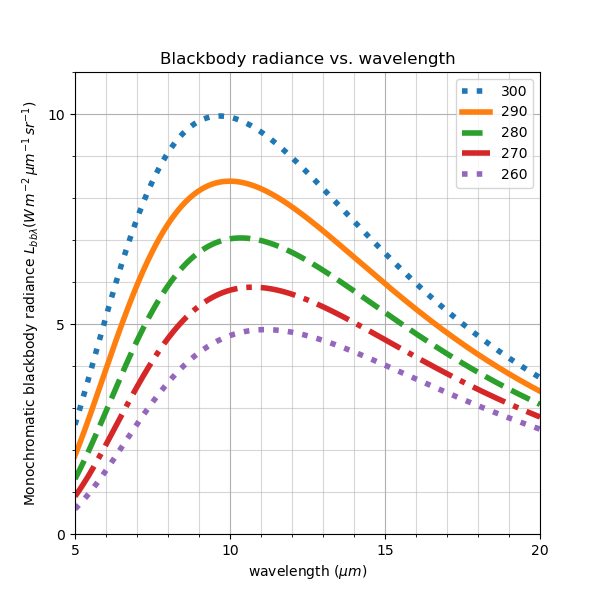
Fig. 6.1 Planck function