19. Zooming an image

• Download zoom_landsat.ipynb from the week3 folder

We need to be able to select a small region of a landsat image to work with. This notebook:downloaded in the week3 folder in the [google drive]

1. zooms in on a 400 pixel wide x 600 pixel high subscene centered on EOS South, using pyproj and the affine transform to map from lon,lat to x,y in UTM zone 10N to row, column in the landsat imag

2. Plots coastlines in the UTM-10N crs

3. Calculates the new affine transform for the subcene, and writes the image out to a 1 Mbyte tiff file using rasterio

4. Repeats the write operation using rioxarray instead of rasterio

• Notable new features

  • Use the pyproj module to find x,y from lat, lon

  • Use numpy slice objects to slice the rows and columns from the image

  • use rioxarray clip_box to clip the desired rows and columns from the image

  • use rasterio and rioxarray to_raster to write a new clipped tif file

import copy
import pprint
from pathlib import Path

import cartopy
import numpy as np
import numpy.random
import rasterio
from affine import Affine
from matplotlib import pyplot as plt
from matplotlib.colors import Normalize
from pyproj import CRS, Transformer
import rioxarray
from cartopy import crs as ccrs

19.1. Get the tiff files and calculate band 5 reflectance

data_dir = Path().home() / 'repos/a301/satdata/landsat'
band_name = 5
data_dir.mkdir(exist_ok=True, parents=True)
disk_file = data_dir / f"hls_landsat8_{band_name}.tif"
has_file = disk_file.exists()

if not has_file:
    raise IOError(f"can't find {disk_file}, rerun with the week2 get_landsat_scene notebook") 
hls_band5 = rioxarray.open_rasterio(disk_file,masked=True)

19.2. Save the crs and the affine transform for the full iamge

We need to keep both full_affine (the affine transform for the full scene, and the coordinate reference system for pyproj (called p_utl below).

Complication – as before, cartopy can’t use the pyproj p_utm, so need to do a convertion for cartopy_crs.

full_affine = hls_band5.rio.transform()
hls_crs = hls_band5.rio.crs.to_wkt()
b5_refl = hls_band5.data.squeeze()*hls_band5.scale_factor

19.3. Convert to cartopy crs for map plot

As in Mapping the landsat scene we’ve got to jump th rough hoops to get the correct cartopy crs. The problem is that hls forgot to put the epsg code in their tif file.

hls_crs

'PROJCS["UTM Zone 10, Northern Hemisphere",GEOGCS["Unknown datum based upon the WGS 84 ellipsoid",DATUM["Not specified (based on WGS 84 spheroid)",SPHEROID["WGS 84",6378137,298.257223563,AUTHORITY["EPSG","7030"]]],PRIMEM["Greenwich",0],UNIT["degree",0.0174532925199433,AUTHORITY["EPSG","9122"]]],PROJECTION["Transverse_Mercator"],PARAMETER["latitude_of_origin",0],PARAMETER["central_meridian",-123],PARAMETER["scale_factor",0.9996],PARAMETER["false_easting",500000],PARAMETER["false_northing",0],UNIT["metre",1,AUTHORITY["EPSG","9001"]],AXIS["Easting",EAST],AXIS["Northing",NORTH]]'

proj_crs = CRS.from_wkt(hls_crs)
pyproj_epsg = proj_crs.to_epsg(min_confidence=60)
print(f"{pyproj_epsg=}")
cartopy_crs = ccrs.epsg(pyproj_epsg)
proj_code = cartopy_crs.to_epsg()
proj_code

pyproj_epsg=32610

32610

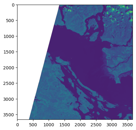
plt.imshow(b5_refl);

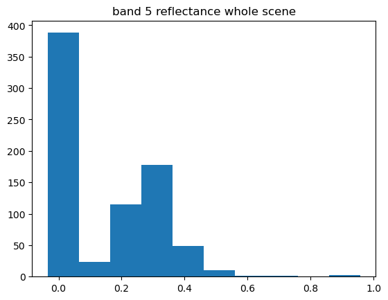
19.3.1. Pick a random selection of 1000 pixels to histogram

Don’t need 3660 x 3660 pixels to get a feeling for the distribution

subset = np.random.randint(0, high=len(b5_refl.flat), size=1000, dtype="l")
plt.hist(b5_refl.flat[subset])
plt.title("band 5 reflectance whole scene")

Text(0.5, 1.0, 'band 5 reflectance whole scene')

19.4. Locate UBC on the map

We need to project the center of campus from lon/lat to UTM 10N x,y using pyproj.Transformer and our crs (which in this case is UTM). We can transform from lat,lon (p_lonlat) to x,y (p_utm) to anchor us to a known point in the map coordinates.

19.4.1. Alert!! the epsg:4326 projection order is (lat, lon) (yikes)

see this stack exchage. Most projections are (lon, lat) which maps more logically to (x, y). Compare the axis order on these two crs:

CRS.from_epsg(proj_code)

<Projected CRS: EPSG:32610>
Name: WGS 84 / UTM zone 10N
Axis Info [cartesian]:
- E[east]: Easting (metre)
- N[north]: Northing (metre)
Area of Use:
- name: Between 126°W and 120°W, northern hemisphere between equator and 84°N, onshore and offshore. Canada - British Columbia (BC); Northwest Territories (NWT); Nunavut; Yukon. United States (USA) - Alaska (AK).
- bounds: (-126.0, 0.0, -120.0, 84.0)
Coordinate Operation:
- name: UTM zone 10N
- method: Transverse Mercator
Datum: World Geodetic System 1984 ensemble
- Ellipsoid: WGS 84
- Prime Meridian: Greenwich

CRS.from_epsg(4326)

<Geographic 2D CRS: EPSG:4326>
Name: WGS 84
Axis Info [ellipsoidal]:
- Lat[north]: Geodetic latitude (degree)
- Lon[east]: Geodetic longitude (degree)
Area of Use:
- name: World.
- bounds: (-180.0, -90.0, 180.0, 90.0)
Datum: World Geodetic System 1984 ensemble
- Ellipsoid: WGS 84
- Prime Meridian: Greenwich

p_utm = CRS.from_epsg(proj_code)
p_latlon = CRS.from_epsg(4326)
transform = Transformer.from_crs(p_latlon, p_utm)
ubc_lon = -123.2460 
ubc_lat = 49.2606
ubc_x, ubc_y = transform.transform(ubc_lat, ubc_lon)
ubc_x,ubc_y

(482101.00635302404, 5456455.217747458)

For more on epsg:4326 see Justyna Jurkowska’s blog entry.

19.5. Locate UBC on the image

Now we need to use the affine transform to go between x,y and col, row on the image. The next cell creates two slice objects that extend on either side of the center point. The tilde (~) in front of the transform indicates that we’re going from x,y to col,row, instead of col,row to x,y. (See this blog entry for reference.) Remember that row 0 is the top row, with rows decreasing downward to the south. To demonstrate, the cell below uses the tranform to calculate the x,y coordinates of the (0,0) corner.

full_ul_xy = np.array(full_affine * (0, 0))
print(f"orig ul corner x,y (km)={full_ul_xy*1.e-3}")

orig ul corner x,y (km)=[ 399.96 5500.02]

19.6. Slice the array

Make our subscene 400 pixels wide and 600 pixels tall, using UBC as a reference point. We need to find the right rows and columns on the image to save for the subscene. Do this by working outward from UBC by a certain number of pixels in each direction, using the inverse of the full_affine transform to go from x,y to col,row

b5_refl.shape[0] - 2230

1430

ubc_col, ubc_row = ~full_affine * (ubc_x, ubc_y)
ubc_col, ubc_row = int(ubc_col), int(ubc_row)
offset_col = 200
offset_row = 300
l_col_offset = -offset_col
r_col_offset = +offset_col
b_row_offset = +offset_row
t_row_offset = -offset_row
col_slice = slice(ubc_col + l_col_offset, ubc_col + r_col_offset)
row_slice = slice(ubc_row + t_row_offset, ubc_row + b_row_offset)
section = b5_refl[row_slice, col_slice]
ubc_ul_xy = full_affine * (col_slice.start, row_slice.start)
ubc_lr_xy = full_affine * (col_slice.stop, row_slice.stop)
ubc_ul_xy, ubc_lr_xy

((476100.0, 5465460.0), (488100.0, 5447460.0))

print(section.shape)

(600, 400)

ubc_col, ubc_row

(2738, 1452)

ubc_x, ubc_y

(482101.00635302404, 5456455.217747458)

full_affine*(ubc_col, ubc_row)

(482100.0, 5456460.0)

upper_left_col = ubc_col + l_col_offset
upper_left_row = ubc_row + t_row_offset
print(upper_left_row, upper_left_col)

1152 2538

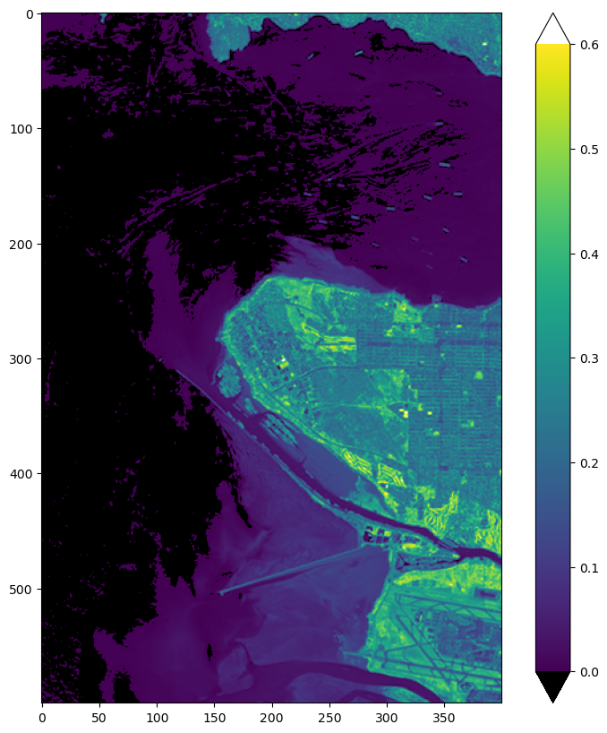
20. Plot the raw band 5 image, clipped to reflectivities below 0.6

This is a simple check that we got the right section. Note that matplotlib ignores the figsize=(10,10) argument in plt.subplots and keeps the correct aspect ratio for the image. I have to make a copy of the palette so my changes “stick”

vmin = 0.0
vmax = 0.6
the_norm = Normalize(vmin=vmin, vmax=vmax, clip=False)
palette = "viridis"
pal = copy.copy(plt.get_cmap(palette))
pal.set_bad("0.75")  # 75% grey for out-of-map cells
pal.set_over("w")  # color cells > vmax red
pal.set_under("k")  # color cells < vmin black
fig, ax = plt.subplots(1, 1, figsize=(10, 10))
cs = ax.imshow(section, cmap=pal, norm=the_norm, origin="upper")
fig.colorbar(cs, extend = 'both');

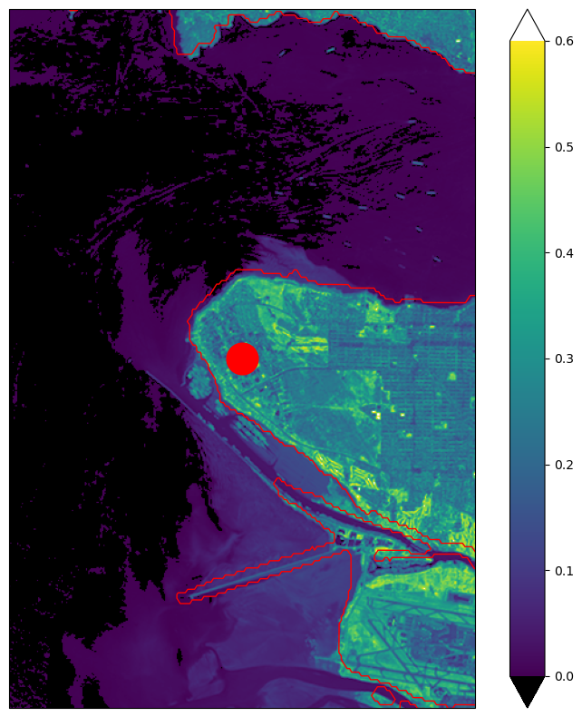
20.1. put this on a map

Cartopy will select the high resoluiton coastline automatically

cartopy_crs

<cartopy._epsg._EPSGProjection object at 0x12b2f2e40>

fig2, ax = plt.subplots(1, 1, figsize=(10,10), subplot_kw={"projection": cartopy_crs})
#
# extent is distance betweenn sides, but the affine transform gives location of pixel centers
# for these tiny pixels it doesn't make a noticeable difference
#
edge_offset = 15 #pxiels are 30 meters wide, so edges are 1/2 a pixel away from centers
image_extent = [ubc_ul_xy[0] - edge_offset, ubc_lr_xy[0] + edge_offset, ubc_lr_xy[1] - edge_offset, ubc_ul_xy[1] + edge_offset]
ax.set_extent(image_extent, crs=cartopy_crs);
cs = ax.imshow(
    section,
    cmap=pal,
    norm=the_norm,
    origin="upper",
    extent=image_extent,
    transform=cartopy_crs,
    alpha=1,
)
ax.add_feature(cartopy.feature.GSHHSFeature(scale="auto", levels=[1, 2, 3],edgecolor='red'))
# shape_project = cartopy.crs.Geodetic()
# ax.add_geometries(
#     df_coast["geometry"], shape_project, facecolor="none", edgecolor="red", lw=2
# )
#ax.coastlines(resolution="10m", color="red", lw=2)
ax.plot(ubc_x, ubc_y, "ro", markersize=25)
fig2.colorbar(cs, extend = 'both');

20.2. Use rasterio to write a new tif file

20.2.1. Set the affine transform for the scene

We can write this clipped image back out to a much smaller tiff file if we can come up with the new affine transform for the smaller scene. Referring again to the writeup we need:

a = width of a pixel
b = row rotation (typically zero)
c = x-coordinate of the upper-left corner of the upper-left pixel
d = column rotation (typically zero)
e = height of a pixel (typically negative)
f = y-coordinate of the of the upper-left corner of the upper-left pixel

which will gives:

new_affine=Affine(a,b,c,d,e,f)

In addition, need to add a third dimension to the section array, because rasterio expects [band,x,y] for its writer. Do this with np.newaxis in the next cell

image_height, image_width = section.shape
ul_x, ul_y = ubc_ul_xy[0], ubc_ul_xy[1]
new_affine = Affine(30.0, 0.0, ul_x, 0.0, -30.0, ul_y)
out_section = section[np.newaxis, ...]
print(out_section.shape)

(1, 600, 400)

20.2.2. Now write this out to band5_clipped_rasterio.tif

Note that the new file does have the utm zone 10 epsg code, since we use the pyproj utm and not the one we got from hls_band5.rio.crs

filename = 'band5_clipped_rasterio.tif'
tif_filename = data_dir / filename
#
# remove the file if it already exists
#
if tif_filename.exists():
    tif_filename.unlink()
num_chans = 1
with rasterio.open(
    tif_filename,
    "w",
    driver="GTiff",
    height=image_height,
    width=image_width,
    count=num_chans,
    dtype=out_section.dtype,
    crs=p_utm,
    transform=new_affine,
    nodata=0.0,
) as dst:
    dst.write(out_section)
    section_profile = dst.profile

print(f"section profile: {pprint.pformat(section_profile)}")

section profile: {'blockxsize': 400,
 'blockysize': 5,
 'count': 1,
 'crs': CRS.from_wkt('PROJCS["WGS 84 / UTM zone 10N",GEOGCS["WGS 84",DATUM["WGS_1984",SPHEROID["WGS 84",6378137,298.257223563]],PRIMEM["Greenwich",0],UNIT["degree",0.0174532925199433,AUTHORITY["EPSG","9122"]],AUTHORITY["EPSG","4326"]],PROJECTION["Transverse_Mercator"],PARAMETER["latitude_of_origin",0],PARAMETER["central_meridian",-123],PARAMETER["scale_factor",0.9996],PARAMETER["false_easting",500000],PARAMETER["false_northing",0],UNIT["metre",1],AXIS["Easting",EAST],AXIS["Northing",NORTH],AUTHORITY["EPSG","32610"]]'),
 'driver': 'GTiff',
 'dtype': 'float32',
 'height': 600,
 'interleave': 'band',
 'nodata': 0.0,
 'tiled': False,
 'transform': Affine(30.0, 0.0, 476100.0,
       0.0, -30.0, 5465460.0),
 'width': 400}

20.3. Repeat the write with rioxarray

We can also write a geotiff with rioxarray. To do that we first need to create the DataArray, then add the attributes, coordinates, affine transform and crs, and then write it out using the to_raster() method

20.3.1. Create the DataArray

In Section 19.6 we used slices to clip the subscene around UBC. For rioxarray, we can use clip_box to do the same thing. We need to provide the bounding box x and y edges we want to clip to, these are given by (ubc_ul_xy, ubc_lr_xy). clip_box wants them in the following order:

(ul_x, lr_y, lr_x, ul_y)

Below we unpack the x,y pairs and then put them into the right order.

ul_x, ul_y = ubc_ul_xy
lr_x, lr_y = ubc_lr_xy
bounding_box = (ul_x, lr_y, lr_x, ul_y)
print(f"{bounding_box=}")

bounding_box=(476100.0, 5447460.0, 488100.0, 5465460.0)

In the call below I’m using the * operator to unpack the tuple

da_band5 = hls_band5.rio.clip_box(*bounding_box)

20.3.1.1. Check the shape, attributes and coordinates

clip_box clips the data, but it also clips the x,y coordinates so that we can still automatically label our image with x and y tick marks

da_band5

<xarray.DataArray (band: 1, y: 600, x: 400)> Size: 960kB
array([[[ 1.200e+01,  1.400e+01, ...,  2.934e+03,  2.916e+03],
        [ 8.000e+00,  1.600e+01, ...,  3.022e+03,  3.004e+03],
        ...,
        [ 5.000e+00, -6.000e+00, ...,  1.748e+03,  2.071e+03],
        [ 8.000e+00,  2.000e+00, ...,  2.397e+03,  2.394e+03]]],
      shape=(1, 600, 400), dtype=float32)
Coordinates:
  * band         (band) int64 8B 1
  * x            (x) float64 3kB 4.761e+05 4.761e+05 ... 4.881e+05 4.881e+05
  * y            (y) float64 5kB 5.465e+06 5.465e+06 ... 5.448e+06 5.447e+06
    spatial_ref  int64 8B 0
Attributes: (12/35)
    ACCODE:                    Lasrc; Lasrc
    arop_ave_xshift(meters):   0, 0
    arop_ave_yshift(meters):   0, 0
    arop_ncp:                  0, 0
    arop_rmse(meters):         0, 0
    arop_s2_refimg:            NONE
    ...                        ...
    ULX:                       399960
    ULY:                       5500020
    USGS_SOFTWARE:             LPGS_15.3.1c
    AREA_OR_POINT:             Area
    scale_factor:              0.0001
    add_offset:                0.0

xarray.DataArray

• band: 1
• y: 600
• x: 400

• 12.0 14.0 14.0 15.0 17.0 ... 2.162e+03 2.479e+03 2.397e+03 2.394e+03

  array([[[ 1.200e+01,  1.400e+01, ...,  2.934e+03,  2.916e+03],
          [ 8.000e+00,  1.600e+01, ...,  3.022e+03,  3.004e+03],
          ...,
          [ 5.000e+00, -6.000e+00, ...,  1.748e+03,  2.071e+03],
          [ 8.000e+00,  2.000e+00, ...,  2.397e+03,  2.394e+03]]],
        shape=(1, 600, 400), dtype=float32)

• Coordinates: (4)
  • band
    (band)
    int64
    1

    array([1])

  • x
    (x)
    float64
    4.761e+05 4.761e+05 ... 4.881e+05

    axis :

    X

    long_name :

    x coordinate of projection

    standard_name :

    projection_x_coordinate

    units :

    metre

    array([476115., 476145., 476175., ..., 488025., 488055., 488085.], shape=(400,))

  • y
    (y)
    float64
    5.465e+06 5.465e+06 ... 5.447e+06

    axis :

    Y

    long_name :

    y coordinate of projection

    standard_name :

    projection_y_coordinate

    units :

    metre

    array([5465445., 5465415., 5465385., ..., 5447535., 5447505., 5447475.],
          shape=(600,))

  • spatial_ref
    ()
    int64
    0

    crs_wkt :

    PROJCS["UTM Zone 10, Northern Hemisphere",GEOGCS["Unknown datum based upon the WGS 84 ellipsoid",DATUM["Not specified (based on WGS 84 spheroid)",SPHEROID["WGS 84",6378137,298.257223563,AUTHORITY["EPSG","7030"]]],PRIMEM["Greenwich",0],UNIT["degree",0.0174532925199433,AUTHORITY["EPSG","9122"]]],PROJECTION["Transverse_Mercator"],PARAMETER["latitude_of_origin",0],PARAMETER["central_meridian",-123],PARAMETER["scale_factor",0.9996],PARAMETER["false_easting",500000],PARAMETER["false_northing",0],UNIT["metre",1,AUTHORITY["EPSG","9001"]],AXIS["Easting",EAST],AXIS["Northing",NORTH]]

    semi_major_axis :

    6378137.0

    semi_minor_axis :

    6356752.314245179

    inverse_flattening :

    298.257223563

    reference_ellipsoid_name :

    WGS 84

    longitude_of_prime_meridian :

    0.0

    prime_meridian_name :

    Greenwich

    geographic_crs_name :

    Unknown datum based upon the WGS 84 ellipsoid

    horizontal_datum_name :

    Not specified (based on WGS 84 spheroid)

    projected_crs_name :

    UTM Zone 10, Northern Hemisphere

    grid_mapping_name :

    transverse_mercator

    latitude_of_projection_origin :

    0.0

    longitude_of_central_meridian :

    -123.0

    false_easting :

    500000.0

    false_northing :

    0.0

    scale_factor_at_central_meridian :

    0.9996

    spatial_ref :

    PROJCS["UTM Zone 10, Northern Hemisphere",GEOGCS["Unknown datum based upon the WGS 84 ellipsoid",DATUM["Not specified (based on WGS 84 spheroid)",SPHEROID["WGS 84",6378137,298.257223563,AUTHORITY["EPSG","7030"]]],PRIMEM["Greenwich",0],UNIT["degree",0.0174532925199433,AUTHORITY["EPSG","9122"]]],PROJECTION["Transverse_Mercator"],PARAMETER["latitude_of_origin",0],PARAMETER["central_meridian",-123],PARAMETER["scale_factor",0.9996],PARAMETER["false_easting",500000],PARAMETER["false_northing",0],UNIT["metre",1,AUTHORITY["EPSG","9001"]],AXIS["Easting",EAST],AXIS["Northing",NORTH]]

    GeoTransform :

    476100.0 30.0 0.0 5465460.0 0.0 -30.0

    array(0)

• Indexes: (3)
  • band
    PandasIndex

    PandasIndex(Index([1], dtype='int64', name='band'))

  • x
    PandasIndex

    PandasIndex(Index([476115.0, 476145.0, 476175.0, 476205.0, 476235.0, 476265.0, 476295.0,
           476325.0, 476355.0, 476385.0,
           ...
           487815.0, 487845.0, 487875.0, 487905.0, 487935.0, 487965.0, 487995.0,
           488025.0, 488055.0, 488085.0],
          dtype='float64', name='x', length=400))

  • y
    PandasIndex

    PandasIndex(Index([5465445.0, 5465415.0, 5465385.0, 5465355.0, 5465325.0, 5465295.0,
           5465265.0, 5465235.0, 5465205.0, 5465175.0,
           ...
           5447745.0, 5447715.0, 5447685.0, 5447655.0, 5447625.0, 5447595.0,
           5447565.0, 5447535.0, 5447505.0, 5447475.0],
          dtype='float64', name='y', length=600))

• Attributes: (35)

  ACCODE :

  Lasrc; Lasrc

  arop_ave_xshift(meters) :

  0, 0

  arop_ave_yshift(meters) :

  0, 0

  arop_ncp :

  0, 0

  arop_rmse(meters) :

  0, 0

  arop_s2_refimg :

  NONE

  cloud_coverage :

  4

  HLS_PROCESSING_TIME :

  2022-03-05T21:45:14Z

  HORIZONTAL_CS_NAME :

  UTM, WGS84, UTM ZONE 10; UTM, WGS84, UTM ZONE 10

  L1_PROCESSING_TIME :

  2020-09-09T04:39:55Z; 2020-09-09T04:39:25Z

  LANDSAT_PRODUCT_ID :

  LC08_L1TP_047025_20150614_20200909_02_T1; LC08_L1TP_047026_20150614_20200909_02_T1

  LANDSAT_SCENE_ID :

  LC80470252015165LGN02; LC80470262015165LGN02

  long_name :

  NIR

  MEAN_SUN_AZIMUTH_ANGLE :

  144.194636459219

  MEAN_SUN_ZENITH_ANGLE :

  29.6215707600637

  MEAN_VIEW_AZIMUTH_ANGLE :

  108.351563730551

  MEAN_VIEW_ZENITH_ANGLE :

  4.81243847783454

  NBAR_SOLAR_ZENITH :

  28.5475827060758

  NCOLS :

  3660

  NROWS :

  3660

  OVR_RESAMPLING_ALG :

  NEAREST

  PROCESSING_LEVEL :

  L1TP; L1TP

  SENSING_TIME :

  2015-06-14T19:00:19.1429430Z; 2015-06-14T19:00:43.0255080Z

  SENSOR :

  OLI_TIRS; OLI_TIRS

  SENTINEL2_TILEID :

  10UDV

  spatial_coverage :

  77

  SPATIAL_RESOLUTION :

  30

  TIRS_SSM_MODEL :

  ACTUAL; ACTUAL

  TIRS_SSM_POSITION_STATUS :

  NOMINAL; NOMINAL

  ULX :

  399960

  ULY :

  5500020

  USGS_SOFTWARE :

  LPGS_15.3.1c

  AREA_OR_POINT :

  Area

  scale_factor :

  0.0001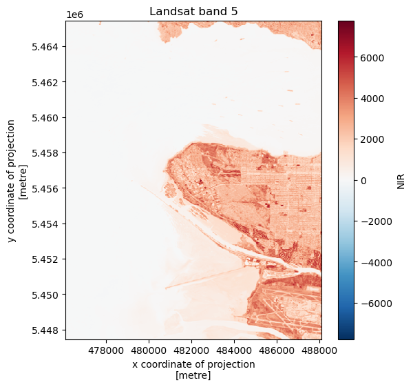

  add_offset :

  0.0

20.3.2. check the image

fig, ax = plt.subplots(1,1, figsize=(6,6))
da_band5.plot(ax=ax)
ax.set_title(f"Landsat band {band_name}");

20.3.3. add the transform and the crs

da_band5.data.dtype

dtype('float32')

da_band5.rio.write_crs(p_utm, inplace=True)
da_band5.rio.write_transform(new_affine, inplace=True);

20.3.4. change some attributes

We need to adjust some of the attributions for the new subscene. To do this, copy the exiting attributes into a dictionary and rewrite the parts you want to change, adding any extras.

new_attrs = da_band5.attrs
new_attrs['ULX']= ul_x
new_attrs['ULY'] = ul_y
band, nrows, ncols = da_band5.shape
new_attrs['NROWS'] = nrows
new_attrs['NCOLS'] = ncols
new_attrs['history'] = "written by the zoom_landsat notebook"
da_band5.rio.update_attrs(new_attrs, inplace = True);

20.3.4.1. check the attributes

da_band5.attrs['history']

'written by the zoom_landsat notebook'

20.3.5. Write out the new geotiff

filename = 'band5_clipped_rio.tif'
filename = data_dir / filename
#
# remove the file if it already exists
#
if tif_filename.exists():
    tif_filename.unlink()
da_band5.rio.to_raster(filename)

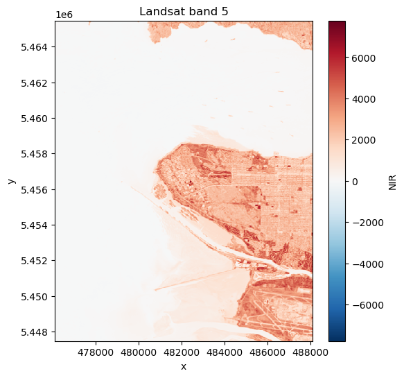
20.3.6. read it back in to check

has_file = filename.exists()
if not has_file:
    raise IOError(f"can't find {filename}, something went wrong above") 
small_band5 = rioxarray.open_rasterio(filename,masked=True)
fig, ax = plt.subplots(1,1, figsize=(6,6))
small_band5.plot(ax=ax)
ax.set_title(f"Landsat band {band_name}");

20.3.6.1. note that we now have the correct epsg code

Because we used the pyproj p_utm crs in our raster write we’ve fixed the missing epsg code problem.

small_band5.rio.crs

CRS.from_wkt('PROJCS["WGS 84 / UTM zone 10N",GEOGCS["WGS 84",DATUM["WGS_1984",SPHEROID["WGS 84",6378137,298.257223563,AUTHORITY["EPSG","7030"]],AUTHORITY["EPSG","6326"]],PRIMEM["Greenwich",0,AUTHORITY["EPSG","8901"]],UNIT["degree",0.0174532925199433,AUTHORITY["EPSG","9122"]],AUTHORITY["EPSG","4326"]],PROJECTION["Transverse_Mercator"],PARAMETER["latitude_of_origin",0],PARAMETER["central_meridian",-123],PARAMETER["scale_factor",0.9996],PARAMETER["false_easting",500000],PARAMETER["false_northing",0],UNIT["metre",1,AUTHORITY["EPSG","9001"]],AXIS["Easting",EAST],AXIS["Northing",NORTH],AUTHORITY["EPSG","32610"]]')