35. Scale heights for typical atmospheric soundings#
Download hydrostatic_balance from the week6 folder
you will also need the new version of a301_lib.py and the soundings folder, all saved to the
same folder as this notebook.
35.1. Plot McClatchey’s US Standard Atmospheres#
There are five different average profiles for the tropics, subarctic summer, subarctic winter, midlatitude summer, midlatitude winter. These are called the US Standard Atmospheres. This notebook shows how to read and plot the soundings, and calculate the pressure and density scale heights.
from matplotlib import pyplot as plt
import matplotlib.ticker as ticks
import numpy as np
from pathlib import Path
import pandas as pd
import pprint
!pwd
/Users/phil/repos/a301_eoas/notebooks/week6
soundings_folder=  Path('./soundings')
sounding_files = list(soundings_folder.glob("*csv"))
print(sounding_files)
[PosixPath('soundings/tropics.csv'), PosixPath('soundings/subsummer.csv'), PosixPath('soundings/subwinter.csv'), PosixPath('soundings/midwinter.csv'), PosixPath('soundings/midsummer.csv')]
35.1.1. Reading the soundings files into pandas#
There are five soundings. The soundings have six columns and 33 rows (i.e. 33 height levels). The variables are z, press, temp, rmix, den, o3den – where rmix is the mixing ratio of water vapor, den is the dry air density and o3den is the ozone density. The units are m, pa, K, kg/kg, kg/m^3, kg/m^3
I will read the 6 column soundings into a pandas (panel data) DataFrame, which is like a matrix except the columns can be accessed by column name in addition to column number. The main advantage for us is that it’s easier to keep track of which variables we’re plotting
name_dict=dict()
sound_dict=dict()
for item in sounding_files:
    name_dict[item.stem]=item
pprint.pprint(name_dict)

for item in sounding_files:
    sound_dict[item.stem]=pd.read_csv(item)
{'midsummer': PosixPath('soundings/midsummer.csv'),
 'midwinter': PosixPath('soundings/midwinter.csv'),
 'subsummer': PosixPath('soundings/subsummer.csv'),
 'subwinter': PosixPath('soundings/subwinter.csv'),
 'tropics': PosixPath('soundings/tropics.csv')}
35.1.2. Use pd.DataFrame.head to see first 5 lines#
for key,value in sound_dict.items():
    print(f"sounding: {key}\n{sound_dict[key].head()}")
sounding: tropics
   Unnamed: 0       z     press   temp     rmix     den         o3den
0           0     0.0  101300.0  300.0  0.01900  1.1670  5.600001e-08
1           1  1000.0   90400.0  294.0  0.01300  1.0640  5.600001e-08
2           2  2000.0   80500.0  288.0  0.00929  0.9689  5.400000e-08
3           3  3000.0   71500.0  284.0  0.00470  0.8756  5.100000e-08
4           4  4000.0   63300.0  277.0  0.00266  0.7951  4.700000e-08
sounding: subsummer
   Unnamed: 0       z     press   temp     rmix     den         o3den
0           0     0.0  101000.0  287.0  0.00910  1.2200  4.900000e-08
1           1  1000.0   89600.0  282.0  0.00600  1.1100  5.400000e-08
2           2  2000.0   79290.0  276.0  0.00420  0.9971  5.600001e-08
3           3  3000.0   70000.0  271.0  0.00269  0.8985  5.800000e-08
4           4  4000.0   61600.0  266.0  0.00165  0.8077  6.000000e-08
sounding: subwinter
   Unnamed: 0       z     press   temp      rmix     den         o3den
0           0     0.0  101300.0  257.1  0.001200  1.3720  4.100000e-08
1           1  1000.0   88780.0  259.1  0.001200  1.1930  4.100000e-08
2           2  2000.0   77750.0  255.9  0.001030  1.0580  4.100000e-08
3           3  3000.0   67980.0  252.7  0.000747  0.9366  4.300000e-08
4           4  4000.0   59320.0  247.7  0.000459  0.8339  4.500000e-08
sounding: midwinter
   Unnamed: 0       z       press   temp     rmix     den         o3den
0           0     0.0  101800.000  272.2  0.00350  1.3010  6.000000e-08
1           1  1000.0   89730.000  268.7  0.00250  1.1620  5.400000e-08
2           2  2000.0   78970.000  265.2  0.00180  1.0370  4.900000e-08
3           3  3000.0   69380.000  261.7  0.00116  0.9230  4.900000e-08
4           4  4000.0   60809.996  255.7  0.00069  0.8282  4.900000e-08
sounding: midsummer
   Unnamed: 0       z     press   temp     rmix     den         o3den
0           0     0.0  101300.0  294.0  0.01400  1.1910  6.000000e-08
1           1  1000.0   90200.0  290.0  0.00930  1.0800  6.000000e-08
2           2  2000.0   80200.0  285.0  0.00585  0.9757  6.000000e-08
3           3  3000.0   71000.0  279.0  0.00343  0.8846  6.200001e-08
4           4  4000.0   62800.0  273.0  0.00189  0.7998  6.400000e-08
We use these keys to get a dataframe with 6 columns, and 33 levels. Here’s an example for the midsummer sounding
midsummer=sound_dict['midsummer']
print(midsummer.head())
list(midsummer.columns)
   Unnamed: 0       z     press   temp     rmix     den         o3den
0           0     0.0  101300.0  294.0  0.01400  1.1910  6.000000e-08
1           1  1000.0   90200.0  290.0  0.00930  1.0800  6.000000e-08
2           2  2000.0   80200.0  285.0  0.00585  0.9757  6.000000e-08
3           3  3000.0   71000.0  279.0  0.00343  0.8846  6.200001e-08
4           4  4000.0   62800.0  273.0  0.00189  0.7998  6.400000e-08
['Unnamed: 0', 'z', 'press', 'temp', 'rmix', 'den', 'o3den']
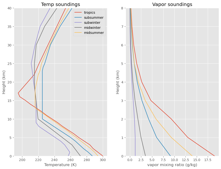
35.1.3. Plot temp and vapor mixing ratio rmix (\(\rho_{H2O}/\rho_{air}\))#
plt.style.use('ggplot')
meters2km=1.e-3
plt.close('all')
fig,(ax1,ax2)=plt.subplots(1,2,figsize=(11,8))
for a_name,df in sound_dict.items():
    ax1.plot(df['temp'],df['z']*meters2km,label=a_name)
    ax1.set(ylim=(0,40),title='Temp soundings',ylabel='Height (km)',
       xlabel='Temperature (K)')

    ax2.plot(df['rmix']*1.e3,df['z']*meters2km,label=a_name)
    ax2.set(ylim=(0,8),title='Vapor soundings',ylabel='Height (km)',
       xlabel='vapor mixing ratio (g/kg)')
ax1.legend();
35.2. Calculating scale heights for temperature and air density#
Here is equation 1 of the Hydrostatic balance notebook:
where
and here is the Python code to do that integral:
g=9.8  #don't worry about g(z) for this exercise
Rd=287.  #kg/m^3
def calcScaleHeight(T,p,z):
    """
    Calculate the pressure scale height H_p

    Parameters
    ----------

    T: vector (float)
      temperature (K)

    p: vector (float) of len(T)
      pressure (pa)

    z: vector (float) of len(T
      height (m)

    Returns
    -------

    Hbar: vector (float) of len(T)
      pressure scale height (m)

    """
    dz=np.diff(z)
    TLayer=(T[1:] + T[0:-1])/2.
    oneOverH=g/(Rd*TLayer)
    Zthick=z[-1] - z[0]
    oneOverHbar=np.sum(oneOverH*dz)/Zthick
    Hbar = 1/oneOverHbar
    return Hbar
Similarly, equation (5) of the Hydrostatic balance notes is:
Which leads to
and the following python function:
def calcDensHeight(T,p,z):
    """
    Calculate the density scale height H_rho

    Parameters
    ----------

    T: vector (float)
      temperature (K)

    p: vector (float) of len(T)
      pressure (pa)

    z: vector (float) of len(T
      height (m)

    Returns
    -------

    Hbar: vector (float) of len(T)
      density scale height (m)
    """
    dz=np.diff(z)
    TLayer=(T[1:] + T[0:-1])/2.
    dTdz=np.diff(T)/np.diff(z)
    oneOverH=g/(Rd*TLayer) + (1/TLayer*dTdz)
    Zthick=z[-1] - z[0]
    oneOverHbar=np.sum(oneOverH*dz)/Zthick
    Hbar = 1/oneOverHbar
    return Hbar
35.2.1. How do \(\overline{H_p}\) and \(\overline{H_\rho}\) compare for the tropical sounding?#
sounding='tropics'
#
# grab the dataframe and get the sounding columns
#
df=sound_dict[sounding]
z=df['z'].values
Temp=df['temp'].values
press=df['press'].values
#
# limit calculation to bottom 10 km
#
hit=z<10000.
zL,pressL,TempL=(z[hit],press[hit],Temp[hit])
rhoL=pressL/(Rd*TempL)
Hbar= calcScaleHeight(TempL,pressL,zL)
Hrho= calcDensHeight(TempL,pressL,zL)
print("pressure scale height for the {} sounding is {:5.2f} km".format(sounding,Hbar*1.e-3))
print("density scale height for the {} is {:5.2f} km".format(sounding,Hrho*1.e-3))
pressure scale height for the tropics sounding is  7.96 km
density scale height for the tropics is  9.74 km
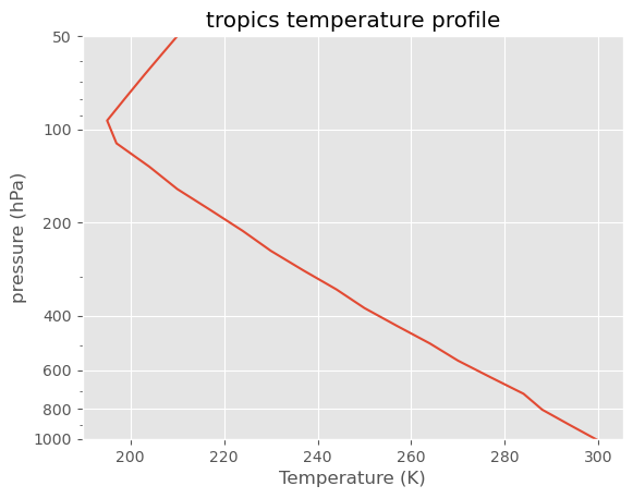
35.2.2. How well do these average values represent the pressure and density profiles?#
theFig,theAx=plt.subplots(1,1)
theAx.semilogy(Temp,press/100.)
#
# need to flip the y axis since pressure decreases with height
#
theAx.invert_yaxis()
tickvals=[1000,800, 600, 400, 200, 100, 50,1]
theAx.set_yticks(tickvals)
majorFormatter = ticks.FormatStrFormatter('%d')
theAx.yaxis.set_major_formatter(majorFormatter)
theAx.set_yticklabels(tickvals)
theAx.set_ylim([1000.,50.])
theAx.set_title('{} temperature profile'.format(sounding))
theAx.set_xlabel('Temperature (K)')
theAx.set_ylabel('pressure (hPa)');
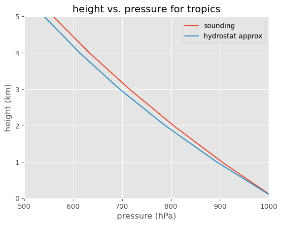
Now check the hydrostatic approximation by plotting the pressure column against
vs. the actual sounding p(T):
fig,theAx=plt.subplots(1,1)
hydroPress=pressL[0]*np.exp(-zL/Hbar)
theAx.plot(pressL/100.,zL/1000.,label='sounding')
theAx.plot(hydroPress/100.,zL/1000.,label='hydrostat approx')
theAx.set_title('height vs. pressure for tropics')
theAx.set_xlabel('pressure (hPa)')
theAx.set_ylabel('height (km)')
theAx.set_xlim([500,1000])
theAx.set_ylim([0,5])
tickVals=[500, 600, 700, 800, 900, 1000]
theAx.set_xticks(tickVals)
theAx.set_xticklabels(tickVals)
theAx.legend(loc='best');
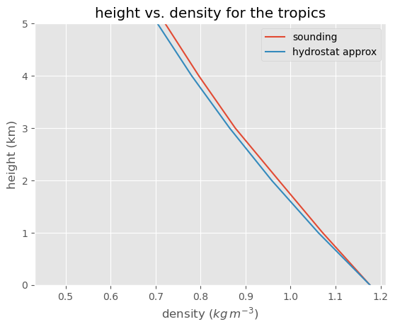
Again plot the hydrostatic approximation
vs. the actual sounding \(\rho(z)\):
fig,theAx=plt.subplots(1,1)
hydroDens=rhoL[0]*np.exp(-zL/Hrho)
theAx.plot(rhoL,zL/1000.,label='sounding')
theAx.plot(hydroDens,zL/1000.,label='hydrostat approx')
theAx.set_title('height vs. density for the tropics')
theAx.set_xlabel(r'density ($kg\,m^{-3}$)')
theAx.set_ylabel('height (km)')
theAx.set_ylim([0,5])
theAx.legend(loc='best');