29. The Schwartzchild Equation

Coverage: Wallace and Hobbs Section 4.5.3 and Stull Chapter 8 p. 225

29.1. Introduction

This note merges material from Wallace and Hobbs p. 135 and equation 4.42

\[\begin{split} \begin{aligned} I_\lambda\left(s_1\right)= & I_{\lambda 0} e^{-\tau_\lambda\left(s_1, 0\right)} \\ & +\int_0^{s_1} k_\lambda \rho r B_\lambda[T(s)] e^{-\tau_\lambda\left(s_1, s\right)} d s \end{aligned} \end{split}\]

with Stull equation 8.3

(29.1)\[ \begin{gathered} L_\lambda = \underbrace{B_\lambda(T_{skin} ) \hat{t}_{tot}}_{\text{surface contribution}} + \underbrace{\sum_{j=1}^n e_{\lambda,j} B_\lambda(T_j) \hat{t}_{\lambda,j}}_{\text{atmospheric contribution}} \end{gathered} \]

Although they don’t look alike, they are two versions of the “Schwartzchild equation” which allow us to calculate the radiance reaching a satellite in an atmosphere that is both absorbing and emitting. Below I’ll use Stull’s notation: \(L\) for radiance and \(e\) for emissivity, but Wallace and Hobbs \(t\) for transmissivity and \(\tau\) for optical depth.

If you go back to Stull Chapter 2 you can see that it involves:

1. the transmissivity \(\hat{t}\) (note that I”ve changed the Stull’s notation to use t instead of \(\tau\))

2. the emissivity e

29.2. Beer’s law

How does this equation relate to Beer’s law, and how would we use it to calculate \(L_\lambda\) reaching a satellite for a particular set of surface/atmosphere conditions?

Where does (29.1) come from? To derive this from the Beer’s law we need to include the fact that the atmosphere is emitting as well as absorbing radiation.

Our previous form of Beer’s law looks like this Beers law – using differentials

(29.2)\[ \frac{dF^\prime}{F^\prime} = \frac{dL^\prime \Delta \omega}{L^\prime \Delta \omega} = d \ln L^\prime = -d (n\,b\,s) = -d \tau^\prime \]

where \(s\ (m)\) is the distance travelled (the path length), \(n\ (\#/m^3)\) is the number denstiy of reflecting/absorbing particles and \(b\ (m^2)\) is the extinction cross section due to absorption only.

Integrating from the surface where \(\tau^\prime=0,\ L^\prime=L_{skin}\) to a vertical height z where \(\tau^\prime = \tau,L^\prime = L\) gives:

\[ \int_{L_{skin}}^L d \ln L^\prime = -\int_0^\tau d\tau^\prime \]

\[ \ln \left ( \frac{L}{L_{skin}} \right ) = - \tau \]

Doing the integral

\[ L = L_{skin} \exp (-\tau) = L_{skin} \hat{t}_{tot} = B_\lambda(T_{skin}) \hat{t}_{tot} \]

where the total transmissivity is:

\[ \hat{t}_{tot} = \exp (-\tau) \]

This is the surface term in (29.1) above, assuming that the surface is radiating like a blackbody at temperature \(T_{skin}\).

29.3. Kirchoff’s Law

Here’s a review of Kirchoff worksheet

The atmosphere isn’t a blackbody, because it’s absorptivity \(a = 1 - \hat{t}\) (no reflection) is not equal to 1 at most wavelengths. Stull p. 41 defines the emissivity e as the fraction of the actual emitted radiance of an object/layer over the radiance a blackbody would emit at the same temperature:

\[ e_\lambda = L_{emitted}/B_\lambda(T) \]

He also says that

\[ a_\lambda = e_\lambda \]

i.e. “good absorbers are good emitters” or Kirchoff’s Law.

To see why this has to be true, consider Section 21, where a blackbody (surface A) is facing a surface B at the same temperature, with absorptivity and emissivity that violate Kirchoff’s law (there is a vacuum between the two plates). Neither surface is transmitting, so surface B is absorbing \(0.6 B_\lambda(T)\) emitted by surface A and emitting \(0.7 B_\lambda(T)\) on its own. Because it is emitting more than it’s absorbed, it has to be cooling, but according to the second law of thermodynamics, objects at the same temperature can’t spontaneously change their temperature without doing work. So we know that \(a_\lambda = e_\lambda\).

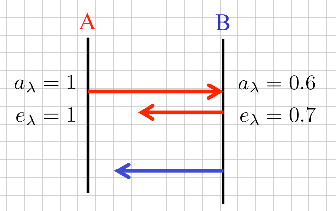
Fig. 29.1 Demonstration of Kirchoff’s law

29.4. Adding emission to Beer’s law

Now include the relationship between \(\hat{t}\), \(\tau\), \(a\) and \(e\):

\[ \hat{t}_\lambda = \frac{L_{\lambda}}{L_{\lambda 0}} = \exp ( - \tau_\lambda) \]

Differentiate this:

(29.3)\[ d \hat{t}_\lambda = d \exp(-\tau_\lambda) = - \exp(-\tau_\lambda)\, d\tau_\lambda = -d\tau_\lambda \]

where we have used the fact that for a thin layer we are expanding about \(\tau = 0\).

Now what about the absorption? Repeat this procedure:

\[ a_\lambda = (1 - \hat{t}_\lambda) \]

Kirchoff says:

\[ e_\lambda = a_\lambda = (1 - \hat{t}_\lambda) \]

So we can use (29.3) to get

\[ de_\lambda = da_\lambda = d(1 - \hat{t}_\lambda) = -d\hat{t}_\lambda = d\tau_\lambda \]

Suppose the layer has constant temperature \(T_{layer}\), then as usual

\[ L_{emission} = e_\lambda B_{\lambda} (T_{layer}) \]

How do we combine this emission with Beer’s law to get the total radiance coming through the top of the layer?

The figure below shows the radiance emitted from the surface and from the thin layer, with their combine contribution to the top of the atmosphere radiance at optical depth \(\tau_T\):

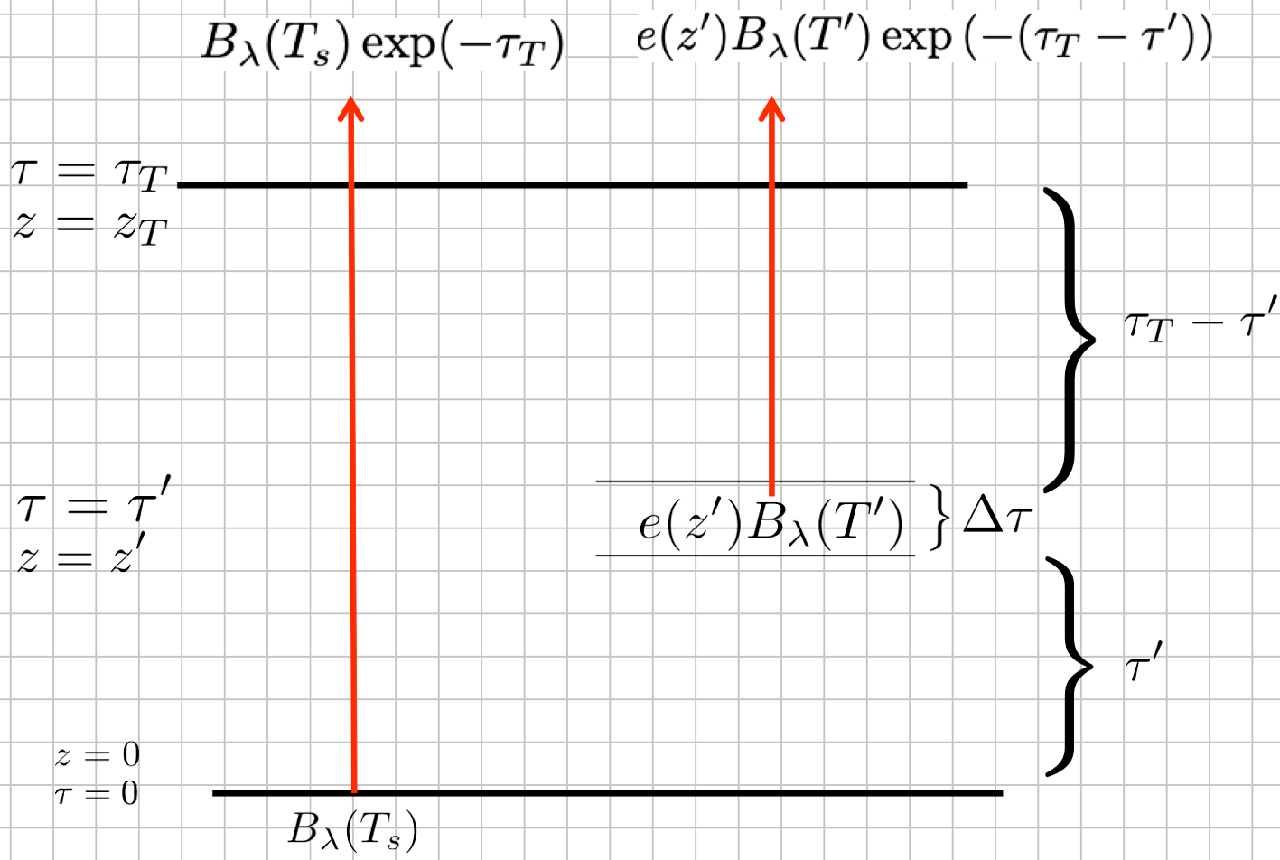
Fig. 29.2 Radiance from an isolated layer and the surface

Before we integrate the entire atmosphere (with temperature changing with height) let’s just integrate the radiance across a layer that is thin enough so we can assume roughly constant temperature.

29.4.1. Constant temperature integration

1. We know the emission from an infinitesimally thin layer:

   (29.4)\[ dL_{emission} = B_{\lambda} (T_{layer}) de_\lambda = B_{\lambda} (T_{layer}) d\tau_\lambda \]

2. Add the gain from \(dL_{emission}\) to the loss from \(dL_{absorption}\) to get the Schwartzchild equation without scattering:

   (29.5)\[ dL_{\lambda,absorption} + dL_{\lambda,emission} = -L_\lambda\, d\tau_\lambda + B_\lambda (T_{layer})\, d\tau_\lambda \]

3. We can rewrite (29.5) as:

   (29.6)\[ \frac{dL_\lambda}{d\tau_\lambda} = -L_\lambda + B_\lambda (T_{layer}) \]

4. In class I used change of variables to derived the following: if the temperature \(T_{layer}\) (and hence \(B_\lambda(T_{layer})\)) is constant with height and the radiance arriving at the base of the layer is \(L_{\lambda 0} = B_{\lambda} T_{skin}\) for a black surface with \(e_\lambda = 1\), then the total radiance exiting the top of the layer is \(L_{\lambda}\) where:

   (29.7)\[ \int_{L_{\lambda 0}}^{L_\lambda} \frac{dL^\prime_\lambda}{L^\prime_\lambda - B_\lambda} = - \int_{0}^{\tau_{T}} d\tau^\prime \]

   Where the limits of integration run from just above the black surface (where the radiance from the surface is \(L_{\lambda 0}\)) and \(\tau=0\) to the top of the layer, (where the radiance is \(L_\lambda\)) and the optical thickness is \(\tau_{\lambda T}\).

29.4.2. Change of variables

To integrate this, make the change of variables:

\[\begin{split} U^\prime &= L^\prime_\lambda - B_\lambda \\ dU^\prime &= dL^\prime_\lambda\\ \frac{dL^\prime_\lambda}{L^\prime_\lambda - B_\lambda} &= \frac{dU^\prime}{U^\prime} = d\ln U^\prime \end{split}\]

where I have made use of the fact that \(dB_\lambda = 0\) since the temperature is constant.

This means that we can now solve this by integrating a perfect differential:

(29.8)\[ \int_{U_0}^U d\ln U^\prime = \ln \left (\frac{U}{U_0} \right ) = \ln \left (\frac{L_\lambda - B_\lambda}{L_{\lambda 0} - B_\lambda} \right ) = - \tau_{\lambda T} \]

Taking the \(\exp\) of both sides:

(29.9)\[ L_\lambda - B_\lambda = (L_{\lambda 0} - B_\lambda) \exp (-\tau_{\lambda T}) \]

or rearranging and recognizing that the transmittance is \(\hat{t_\lambda} = \exp(-\tau_{\lambda T} )\):

(29.10)\[ L_\lambda = L_{\lambda 0} \exp( -\tau_{\lambda T} ) + B_\lambda (T_{layer})(1- \exp( -\tau_{\lambda T} )) \]

\[ L_\lambda = L_{\lambda 0} \hat{t}_{\lambda} + B_\lambda (T_{layer})(1- \hat{t}_{\lambda}) \]

\[ L_\lambda = L_{\lambda 0} \hat{t}_{\lambda} + B_\lambda (T_{layer})a_\lambda \]

1. so bringing in Kirchoff’s law, the radiance exiting the top of the isothermal layer of thickness \(\Delta \tau\) is:

\[ L_\lambda = L_{\lambda 0} \hat{t}_{\lambda} + e_\lambda B_\lambda \]

29.5. Temperature changing with height

29.5.1. Getting to Stull 8.3

To get Stull’s eq. 8.3 (our (29.1)), we need integrate (29.6) when temperature and therefor \(B_\lambda(T)\) is changing with height.

• Here’s the Schwartzchild equation again:

(29.11)\[ \frac{dL_\lambda}{d\tau_\lambda}= - L_{\lambda} + B_\lambda \]

• Now with \(T\) changing with height, we need to use an integrating factor to solve this. Essentially this means multiplying both sides by \(exp(\tau)\) so that we’re in the position to integrate a perfect differential:

• Specifically, look at how the chain rule works for the product \(L\exp(\tau)\) :

(29.12)\[ d(L\exp(\tau))=\exp(\tau)dL + L\exp(\tau)d\tau \]

• Now multiply both sides of (29.11) by \(exp(\tau)\):

(29.13)\[ \exp(\tau) dL_\lambda + L_\lambda \exp(\tau)\,d\tau=\exp(\tau)B_\lambda(T) \,d\tau \]

• Next use use the chain rule in reverse to combine the two terms on the left, and integrate:

  \[ d\left( L_\lambda\exp(\tau)\right )=\exp(\tau)B_\lambda d\tau \]
  (29.14)\[ \int_0^{\tau}d(L^\prime_\lambda\exp(\tau^\prime))=\int_0^{\tau} \exp(\tau^\prime)B^\prime_\lambda d\tau^\prime \]

• Impose the boundary condition that at \(\tau^\prime=0\):

  \[\begin{split} \begin{gathered} L^\prime_\lambda=B_\lambda(T_{skin})\\ \hat{t}_\lambda=\exp(0)=1 \end{gathered} \end{split}\]

• Which means that when we integrate (29.14) we get:

  \[ L_\lambda\exp(\tau) - B_\lambda(T_{skin}) = \int_0^{\tau} \exp(\tau^\prime)B_\lambda(T^\prime) d\tau^\prime\nonumber \]

• Dividing through by \(\exp(\tau)\) we get:

  (29.15)\[ L_\lambda(\tau)= B_\lambda(T_{skin})( \exp(-\tau) + \int_0^{\tau} \exp\left( - (\tau -\tau^\prime) \right ) B_\lambda(T)\, d\tau^\prime \]

• Equation (29.15) works for any height in the atmosphere. For the particular case at the top of the atmosphere where \(\tau = \tau_{\lambda T}\) we have

  (29.16)\[ L_\lambda(\tau_{\lambda T})= B_\lambda(T_{skin})( \exp(-\tau_{\lambda T}) + \int_0^{\tau} \exp\left( - (\tau_{\lambda T} -\tau^\prime) \right ) B_\lambda(T)\, d\tau^\prime \]

• Compare (29.16) to Stull 8.3, which is:

  (29.17)\[ \begin{gathered} L_\lambda = B_\lambda(T_{skin} ) \hat{t}_{tot} + \sum_{j=1}^n e_\lambda B_\lambda(T_j) \hat{t}_{\lambda,j} \end{gathered} \]

  We can connect (29.17) and (29.16) if we recognize that

  \[ \hat{t}_{\lambda,j} = \exp\left( -(\tau_{\lambda T} -\tau_j) \right ) \]

  i.e. \(\hat{t}\) is the transmission from layer j to the top of the atmosphere and also that the layers are thin enough so that we can make the approximation that:

  \[ e_\lambda = de_\lambda = d\tau^\prime \]

29.5.2. Getting to Stull 8.4

• Equation 8.4 on p. 225 says:

  (29.18)\[ \begin{gathered} L_\lambda = B_\lambda(T_{skin}) \hat{t}_{\lambda,tot} + \sum_{j=1}^n B_\lambda(T_j) \Delta \hat{t}_{\lambda,j} \end{gathered} \]

• What happened to \(e_\lambda(z_j)\) and \(\hat{t}_{\lambda,j}\) from (29.17)? To see why this works, go back to the exact solution (29.16) and use the definition \(\hat{t} = \exp\left( -(\tau_{\lambda T} -\tau^\prime) \right )\)

  (29.19)\[ L_\lambda(\tau_{\lambda T})= B_\lambda(T_{skin})( \exp(-\tau_{\lambda T}) + \int_0^{\tau} B(T)\, \hat{t} \, d\tau^\prime \]

  Now recognize that you can do the following differential:

  (29.20)\[ d\hat{t} = \frac{ d\hat{t}_{j} }{d\tau^\prime}\, d \tau^\prime = \exp\left( -(\tau_{\lambda T} -\tau^\prime)\right ) d \tau^\prime = \hat{t}\, d\tau^\prime \]

  So insert (29.20) into (29.19) to get

  (29.21)\[ L_\lambda(\tau_{\lambda T})= B_\lambda(T_{skin}) \exp(-\tau_{\lambda T}) + \int_0^{\tau_{\lambda T}} B_\lambda(T)\, d\hat{t} \]

  Which is just the calculus version of (29.18). The \(\Delta \hat{t}\) term in (29.18) is called the “weighting function”, defined by

  (29.22)\[ \Delta \hat{t} = \exp\left( -(\tau_{\lambda T} -\tau^\prime) \right ) \Delta \tau^\prime \]

  • Question: notice that as we make \(\Delta \tau^\prime\) thicker in (29.22) the transmissivity \(\Delta \hat{t}\) becomes larger – why does this make sense?

29.6. Why do we care?

We care because if we know T(z) and \(\tau(z)\) as a function of height we can use (29.22) to calculate the weighting function \(\Delta \hat{t}_\lambda\) and find the radiance \(L_\lambda\) at the satellite using (29.18). Alternatively, if we measure \(L_\lambda\) from satellites we can say something about T(z) and \(\tau(z)\)