49. Working with surface class data

49.1. Introduction

This notebook uses land classification data from the Impact Observatory:

https://docs.impactobservatory.com/lulc-maps/maps-for-good.html

The land use/land classification process assigns a category between 0-11 for the following 9 categories (they have combined former categories 3 and 6 in the the category 11 (rangeland).

\[\begin{split} \begin{array}{|ll|} \hline 0 & \text { No data } \\ \hline 1 & \text { Water } \\ \hline 2 & \text { Trees } \\ \hline 4 & \text { Flooded Vegetation } \\ \hline 5 & \text { Crops } \\ \hline 7 & \text { Built Area } \\ \hline 8 & \text { Bare Ground } \\ \hline 9 & \text { Snow/lce } \\ \hline 10 & \text { Clouds } \\ \hline 11 & \text { Rangeland } \\ \hline \end{array} \end{split}\]

It’s distributed as a tiff file for a particular UTM zone. To download the file for your region, first visit https://docs.impactobservatory.com/tutorials/aws-open-data-exchange/aws-open-data-exchange.html and read the instructions for how to use the stac-browser to select areas and time periods (the files have been updated every year from 2017 to 2023). From there select the filter box on the right hand side and filter on area and time. You should get a file offered for each of the 6 years of data.

49.2. Installation

• Download the rio_land_classification.ipynb file from the week9 folder

• To run this notebook, you’ll also need to move 2 files from the downloads/vancouver_2023 folder to your ~/repos/a301/satdata/landsat/vancouver_2023 folder: clipped_band5.tif (which contains the bounding box we need to clip to) and the UTM Zone 10N classified tif file for 2023: 10U_2023.tif (137 Mbytes)

from pathlib import Path
import json

import cartopy
import rasterio
import pyproj
import numpy as np
from matplotlib import pyplot as plt
import rioxarray
import xarray as xr
from cartopy import crs as ccrs
    

49.3. Get the path to the clipped scene

We only need the bounding box and from affine transform from this tif file so we can clip the classification data to our Vancouver region, and use rio.reproject_match to resample the 10 meter classification pixels onto the 30 meter landsat grid.

data_dir = Path().home() / 'repos/a301/satdata/landsat'
the_tif = list(data_dir.glob('**/vancouver_2023/clipped_band5.tif'))[0]
print(the_tif)

/Users/phil/repos/a301/satdata/landsat/vancouver_2023/clipped_band5.tif

49.4. Read landsat band 5 bounds

landsat_nir = rioxarray.open_rasterio(the_tif,mask_and_scale=True)
landsat_nir = landsat_nir.squeeze()
landsat_nir.shape

(1000, 800)

landsat_crs = pyproj.CRS(landsat_nir.rio.crs)
landsat_bounds = landsat_nir.rio.bounds()

49.5. Read and clip the surface classification

This file needs to be clipped before we can do anything, because it’s so big.

the_tif = list(data_dir.glob('**/vancouver_2023/10U*2023*tif'))[0]
print(the_tif)

/Users/phil/repos/a301/satdata/landsat/vancouver_2023/10U_2023.tif

land_class = rioxarray.open_rasterio(the_tif)
land_class = land_class.squeeze()

land_class.shape,land_class.dtype

((89383, 44754), dtype('uint8'))

clipped_class = land_class.rio.clip_box(*landsat_bounds)

Note that the clipped classifcation is 3 times as large as landsat 1000 x 800 pixel scene.

clipped_class.shape

(3000, 2400)

49.6. reproject clipped_class onto the landsat band 5 grid

We want exactly the same grid as landsat, which means that we need to turn 3x3 groups of 10 meter classifier pixels into a 30 x 30 meter landsat pixel. We don’t want to average the classification categories together, because that would be meaningless, so instead well take the mode of the 9 pixels and assign that most prevalent category to the larger landsat pixel.

Rasterio specifies the various resampling strategies using python enums, which are kept in the rasterio.enum.Resampling module. Enums are a more robust way to specify integer choices. In fact Resampling.mode is really just the number 6.

from rasterio.enums import Resampling
Resampling.mode

<Resampling.mode: 6>

49.7. Run the resampler using reproject_match

matched_class = clipped_class.rio.reproject_match(landsat_nir,
                                                  resampling=Resampling.mode)
matched_class.shape

(1000, 800)

49.7.1. Set water values to np.nan

We need to change from bytes to floats to do this, since np.nan is a floatl

matched_class = matched_class.astype(np.float32)
matched_class.data[matched_class.data == 1] = np.nan

49.7.2. How many pixels are crops?

np.sum(matched_class.data == 5)

np.int64(965)

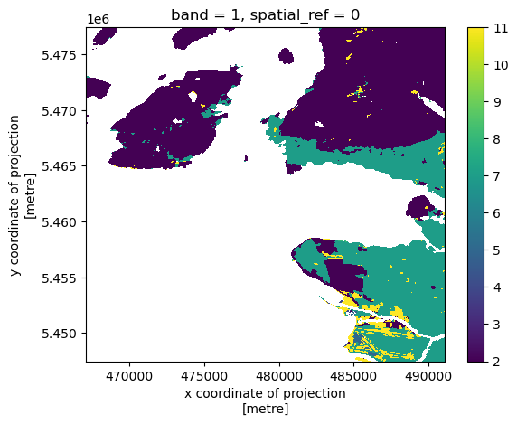
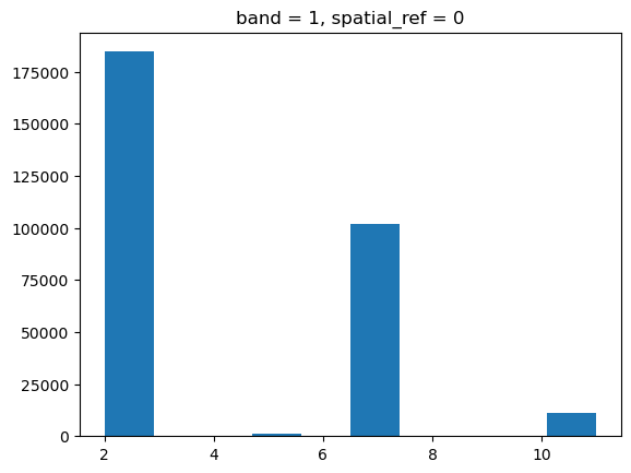
49.8. Dominant categories

As expected, lots of trees (2) and build area (7) with some sand/road/runway pixels misclassified as clouds (10)

matched_class.plot.hist();

matched_class.plot.imshow();