55. Assignment 6 solution

Upload a pdf and a notebook for the following problems:

55.1. Q1 Planck wavenumber

Planck’s law as a function of wavelength:

(55.1)\[ B_\lambda(\lambda, T)=\frac{2 h c^2}{\lambda^5} \frac{1}{e^{h c /\left(\lambda k_{\mathrm{B}} T\right)}-1} \]

Use change of variables to rewrite (46.1) in terms of wavenumber \(\tilde{\nu} = 1/\lambda\) and show that it is:

(55.2)\[ B_{\tilde{\nu}}(\tilde{\nu}, T)=2 h c^2 \tilde{\nu}^3 \frac{1}{e^{h c \tilde{\nu} /\left(k_{\mathrm{B}} T\right)}-1} \]

55.1.1. Q1 solution

We want to change variables for the definite integral:

\[ \int_{\lambda_1}^{\lambda_2} B_\lambda d\lambda = \int_{\tilde{\nu_1}}^{\tilde{\nu_2}} B_{\tilde{\nu}}d{\tilde{\nu}} \]

where \(\lambda = 1/\tilde{\nu}\). We know that the two integrals are equal because they have to integrate to the same flux in \(W\,m^{-2}\).

First, make the substitution in \(B_\lambda\):

\[ B_{\tilde{\nu}}: 2 h c^2 \tilde{\nu}^5 \frac{1}{e^{h c \tilde{\nu} /\left( k_{\mathrm{B}} T\right)}-1} \]

Now add \(d\tilde{\nu}\) given that:

\[ d\lambda = d \left ( \frac{1}{\tilde{\nu}} \right ) = -\tilde{\nu}^{-2} d\tilde{\nu} \]

So the integral become:

\[ \int_{\tilde{\nu_1}}^{\tilde{\nu_2}} B_{\tilde{\nu}}(\tilde{\nu}, T)d{\tilde{\nu}} = \int_{\tilde{\nu_1}}^{\tilde{\nu_2}} 2 h c^2 \tilde{\nu}^5 \frac{1}{e^{h c \tilde{\nu} /\left(k_{\mathrm{B}} T\right)}-1} (-\tilde{\nu}^{-2}) d\tilde{\nu} \]

To get rid of the minus sign, recognize that if \(d\lambda > 0\), then \(d\tilde{\nu} < 0\) since \(\tilde{\nu_1} > \tilde{\nu_2}\) which means that we flip the limits of integration to proceed in a positive \(\tilde{\nu}\) direction and the integral is:

\[ \int_{\tilde{\nu_2}}^{\tilde{\nu_1}} B_{\tilde{\nu}}(\tilde{\nu}, T)d{\tilde{\nu}} = \int_{\tilde{\nu_2}}^{\tilde{\nu_1}} 2 h c^2 \tilde{\nu}^3 \frac{1}{e^{h c \tilde{\nu} /\left(k_{\mathrm{B}} T\right)}-1} d\tilde{\nu} \]

55.2. Q2 Stefan-Boltzman

Integrate

(55.3)\[ \int_0^\infty B_{\tilde{\nu}}(\tilde{\nu}, T)d \tilde{\nu}=2 h c^2 \int_0^\infty \frac{\tilde{\nu}^3}{e^{h c \tilde{\nu} /\left(k_{\mathrm{B}} T\right)}-1}\,d \tilde{\nu} \]

to find the Stefan-Boltzman equation given that

(55.4)\[ \int_0^\infty \frac{u^3}{(e^u -1 )} du = \frac{\pi^4}{15} \]

(Riemann zeta function)

i.e. show that:

\[ \int_0^\infty B_{\nu} d\nu = \frac{\sigma}{\pi} T^4 \]

where

\[ \sigma=\frac{2 \pi^5 k_B^4}{15 c^2 h^3} \]

55.2.1. Q2 Answer

Make the following substitution:

\[ u = \frac{hc\tilde{\nu}}{k_B T} \]

so:

\[ \tilde{\nu} = \frac{k_B T u}{hc} \]

\[ (2hc^2)\,\tilde{\nu}^3 = (2hc^2)\,\frac{k_B^3 T^3 u^3}{h^3c^3}=\frac{2 \pi^4 k_B^4}{15 c^2 h^3} \]

\[ d\tilde{\nu} = \frac{k_B T}{hc}dU \]

\[ 2 h c^2 \int_0^\infty \frac{\tilde{\nu}^3}{e^{h c \tilde{\nu} /\left(k_{\mathrm{B}} T\right)}-1}\,d \tilde{\nu} = \frac{2 k_B^3T^3}{h^2 c} \frac{k_B T}{hc} \int_0^\infty \frac{u^3}{(e^u - 1)} du = \frac{2 k_B^3T^3}{h^2 c} \frac{k_B T}{hc} \frac{\pi^4}{15} = \frac{2 \pi^4 k_B^4}{15 c^2 h^3} T^4 \]

55.3. Q3 Wien’s law

Show that the maximum value for

(55.5)\[ B_\lambda(\lambda, T)=\frac{2 h c^2}{\lambda^5} \frac{1}{e^{h c /\left(\lambda k_{\mathrm{B}} T\right)}-1} \]

occurs at:

\[ \lambda_{max} \propto \frac{1}{T} \]

(Wien’s law)

55.3.1. Q3 Answer

As shown below, we are working with parameters for which \(e^u\), where \(u=h c /\left(\lambda k_B T\right ) \approx e^5 \approx 150 \gg 1\) so it’s safe to write:

(55.6)\[ B_\lambda(\lambda, T) \approx \frac{2 h c^2}{\lambda^5} \frac{1}{e^{h c /\left(\lambda k_{\mathrm{B}} T\right)}} = a \lambda^{-5}\exp(-b/(\lambda T)) \]

We want to find \(\lambda_{max}\) the wavelength at which \(\frac{dB}{d\lambda} = 0\).

Use the chain rule on (55.6):

\[ \frac{dB}{d\lambda} = a (-5 \lambda^{-6})\exp(-b/(\lambda T)) + a \lambda^{-5} \exp(-b/(\lambda T) (b/(\lambda^2 T) =0 \]

Simplify:

\[ -5\lambda^{-1} + b\lambda^{-2}/T = 0 \]

\[ 5 = \frac{b \lambda^{-1}}{T} \]

\[ \lambda_{max} = \frac{b}{3T} \]

import numpy as np
#
#
#
#
# From the Planck notebook
#
c=2.99792458e+08  #m/s -- speed of light in vacuum
h=6.62606876e-34  #J s  -- Planck's constant
kb=1.3806503e-23  # J/K  -- Boltzman's constant
#
# Try T = 5800 K and the_lambda = 5.e-7 m (solar radiation, green light
#
T = 5800
the_lambda = 5.e-7
u = h*c/(the_lambda*kb*T)
print(f"shortwave {u=:8.2f}")
#
# Try T = 300 K and the_lambda = 10.e-6 m (earth radiation, longwave
#
T = 300
the_lambda = 10.e-6
u = h*c/(the_lambda*kb*T)
print(f"longwave {u=:8.2f}")
print(f"{np.exp(5)=:.1f}")

shortwave u=    4.96
longwave u=    4.80
np.exp(5)=148.4

55.4. Q4 Radar Rainrate

55.4.1. Analytic

Integrate \(Z=\int D^6 n(D) dD\) on paper, assuming a Marshall Palmer size distribution and show that it integrates to:

\[ Z \approx 300 RR^{1.5} \]

with Z in \(mm^6\,m^{-3}\) and RR in mm/hr. It’s helpful to know that:

\[ \int^\infty_0 x^n \exp( -a x) dx = n! / a^{n+1} \]

55.4.2. Q4 Analytic Answer

\[ n(D) = n_0 \exp(-4.1 RR^{-0.21} D ) \]

with \(n_0=8000\) in units of \(m^{-3}\,mm^{-1}\), D in mm, so that \(\Lambda=4.1 RR^{-0.21}\) has to have units of \(mm^{-1}\).

If we use this to integrate:

\[ Z=\int D^6 n(D) dD \]

and use the hint that

\[ \int^\infty_0 x^n \exp( -a x) dx = n! / a^{n+1} \]

with n=6, a=\(\Lambda\) we get:

\[ Z=\frac{n_0\, 6!}{\Lambda^7} \]

with units of \(m^{-3}\,mm^{-1}/(mm^{-1})^7=mm^6\,m^{-3}\) as required. Since \(n_0=8000\,m^{-3}\,mm^{-1}\) and 6!=720, the numerical coeficient is \(8000x720/(4.1**7)=295.75\) and \((RR^{-0.21})^{-7} = RR^{1.47}\) so the final form is:

\[ Z=296 RR^{1.47} \]

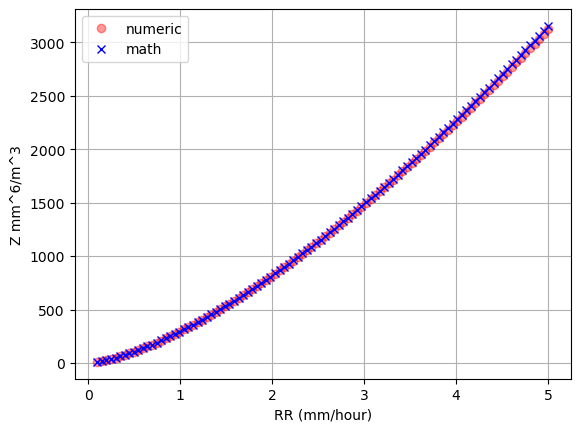
55.5. Q5 Radar Rainrate Python

Repeat using numerical integration in python (i.e. np.diff and np.sum) and show that the result agrees.

import numpy as np
from matplotlib import pyplot as plt
#
# Marshall Palmer distribution
#
def calc_num_dist(Dvals,RR,n0=8000):
    the_dist = n0*np.exp(-4.1*RR**(-0.21)*Dvals)
    return the_dist

Dvals = np.linspace(0.01,5,1000)
dD = np.diff(Dvals)
#
# need the midpoint diameters for the rectangular integration
#
Dmid = (Dvals[1:] + Dvals[0:-1])/2.

#
# loop over 100 rain rates
#
RRvals = np.linspace(0.1,5,100)

#
# Brute force integration
#
Zvals = []
for the_RR in RRvals:
    num_dist = calc_num_dist(Dvals,the_RR)
    bin_heights = (num_dist[1:] + num_dist[0:-1])/2.
    theZ = np.sum(Dmid**6.*bin_heights*dD)
    Zvals.append(theZ)
    
fig, ax = plt.subplots(1,1)
ax.plot(RRvals,Zvals,'ro',alpha=0.4,label='numeric')
Z_math = 296*RRvals**1.47
ax.plot(RRvals,Z_math,'bx',label="math")
ax.set(xlabel="RR (mm/hour)",ylabel="Z mm^6/m^3")
ax.grid(True)
ax.legend(loc='best');