33. Cartopy mapping Buenos Aires

In order to run this notebook go to the download folder and get

• week5/cartopy_mapping_buenos_aires.ipynb

• week5/a301_lib.py

• buenos_aires/*B02.tif

the band2 (blue) tif needs to be in ~/repos/a301/satdata/landsat/buenos_aires/.

33.1. Introduction

This notebook shows how to turn a Landsat Zone North UTM crs into a Zone South crs so that we can use cartopy. Basically, all we need to do is to add a “false northing” of 10,000,000 meters to the upper left corner of the raster image, as it is defined in the affine transform that is stored in the geotiff metadata. Once we have the Zone 21S transform, we can use it to find the image extent that cartopy needs to plot the raster along with the coastline.

33.2. Example

Use Buenos Aires as a specifc test.

Google says Buenos Aires in in UTM zone 21 South, with an epgs code of 32721

lat = -34.6037 deg S lon = -58.3816 deg W

We want to put an image on a map, with this Landsat scene

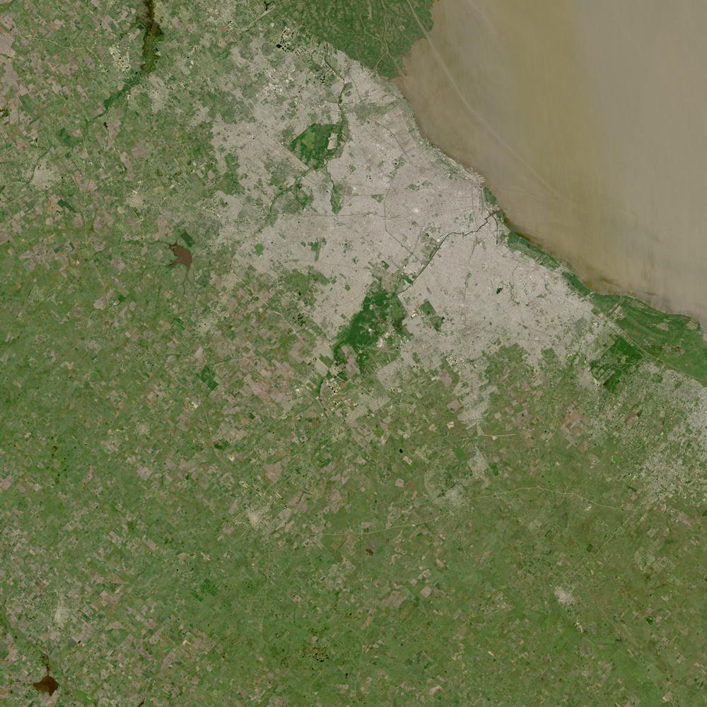
Fig. 33.1 Landsat browse image of Buenos Aires

33.3. Import libraries

The file a301_lib.py is a new python module containing course code. For week 5 it contains rowcol2latlon from Getting lat,lon from row, column and make_pal from Adding a palette to an axis. We use the make_pal function below

from a301_lib import make_pal

import cartopy.crs as ccrs
import matplotlib.pyplot as plt
import cartopy
from pathlib import Path
import rioxarray
import affine

from matplotlib import pyplot as plt
from matplotlib.colors import Normalize
import warnings

silence weird cartopy geojson warnings (doesn’t seem to help)

warnings.filterwarnings("ignore")

33.4. Set up the UTM CRS for Zone 21S

Here is the center of buenos aires

ba_lat = -34.6037 # deg N
ba_lon = -58.3816 # deg E

33.4.1. The epsg code for Zone 21S is 32721

geodetic = ccrs.Geodetic()
the_crsS = ccrs.epsg(32721)
ba_x, ba_yS = the_crsS.transform_point(ba_lon, ba_lat, geodetic)
print(f"{ba_x=:.0f}, {ba_yS=:.0f}")

ba_x=373318, ba_yS=6170036

33.5. Repeat this for UTM Zone 21N

This has an epsg code of 32621

the_crsN = ccrs.epsg(32621)
ba_x, ba_yN = the_crsN.transform_point(ba_lon, ba_lat, geodetic)
print(f"{ba_x=:.0f}, {ba_yN=:.0f}")

ba_x=373318, ba_yN=-3829964

33.6. False northing

Zone 21 North has negative y values south of the equator. To eliminate this, someone decided to create a new zone, Zone 21 South, by adding 10,000,000 meters to every y value south of the equator, the “false northing”.

You can see this when you subtract the y for Buenos Aires in 201N from the y in 21S:

print(f"false northing: {(ba_yS - ba_yN)=:.0f} meters")

false northing: (ba_yS - ba_yN)=10000000 meters

33.6.1. Zone 21S ends at 80 deg S

see the epsg website

What is the most southern y point in Zone 21N coordinates?

Note that the x coords are identical in both projections, but

sp_yS - sp_yN = 10,000,000

sp_lon = -57. # zone 21 central meridian 57 deg W
sp_lat = -80  #farthest south point
sp_x, sp_yN = the_crsN.transform_point(sp_lon, sp_lat, geodetic)
print(f"{(sp_x,sp_yN)=}")

(sp_x,sp_yN)=(np.float64(500000.00000000023), np.float64(-8881585.815988095))

33.6.2. How about Zone 21S

sp_x, sp_yS = the_crsS.transform_point(sp_lon, sp_lat, geodetic)
print(f"{(sp_x,sp_yS)=}")
print(f"{(sp_yS - sp_yN)=}")

(sp_x,sp_yS)=(np.float64(500000.00000000023), np.float64(1118414.1840119045))
(sp_yS - sp_yN)=np.float64(10000000.0)

33.6.3. How about the equator?

eq_lon = -57. # zone 21 central meridian 57 deg W
eq_lat = 0  #farthest north point
eq_x, eq_yS = the_crsS.transform_point(eq_lon, eq_lat, geodetic)
print(f"{(eq_x,eq_yS)=}")
eq_x, eq_yN = the_crsN.transform_point(eq_lon, eq_lat, geodetic)
print(f"{(eq_x,eq_yN)=}")

(eq_x,eq_yS)=(np.float64(500000.0000000014), np.float64(10000000.0))
(eq_x,eq_yN)=(np.float64(500000.0000000014), np.float64(0.0))

So there’s a 10 million meter discontinuity when you change zones at the equator. NASA decided this was a problem, and did away with the false northing, permitting negative y values for Zone 21N. Cartopy disagreed, and requires positive y values in each utm zone.

33.7. Draw a Buenos Aires map with the_CRSS south CRS

follow Mapping Vancouver with cartopy

make it 50 x 50 km with BA in the center

#
# pick a bounding box in map coordinates
# set the extent for 25 km in each direction from BA
#
half_width = 25*1.e3  # 50,000 m
xleft, xright = ba_x - half_width, ba_x + half_width
ybot, ytop =  ba_yS - half_width, ba_yS + half_width
extent = [xleft, xright, ybot, ytop]

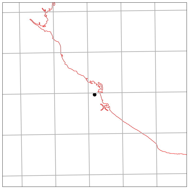
fig, ax = plt.subplots(1, 1, figsize=(10, 10), subplot_kw={"projection": the_crsS})
ax.set_extent(extent, the_crsS)
ax.plot(ba_x, ba_yS, "ko", markersize=10)
ax.gridlines(linewidth=2)
ax.add_feature(cartopy.feature.GSHHSFeature(scale="auto", edgecolor = "red", levels=[1, 2, 3]));

33.8. Now overlay a landsat image

We need to take the affine transform from the landsat image and change it from zone 21N to 21S. To do that we need to rewrite the upper-left corner Y value by adding 10,000,000 meters to it.

data_dir = Path().home() / 'repos/a301/satdata/landsat/buenos_aires'
the_tif = list(data_dir.glob('**/HLS.L30*B02.tif'))[0]
print(the_tif)

/Users/phil/repos/a301/satdata/landsat/buenos_aires/HLS.L30.T21HUB.2015340T134445.v2.0.B02.tif

33.8.1. Grab the affine transform

Recall from Mapping the landsat scene that the affine transform handles the conversion from x, y to row, column and back. The transform stored in the landsat images is written with Z 21N. We need to turn that transform into 21S by add 10,000,000 m to the y value of the upper left corner.

The layout for the transform is:

a = width of a pixel
b = row rotation (typically zero)
c = x-coordinate of the upper-left corner of the upper-left pixel
d = column rotation (typically zero)
e = height of a pixel (typically negative)
f = y-coordinate of the of the upper-left corner of the upper-left pixel

So f is the value we need to change.

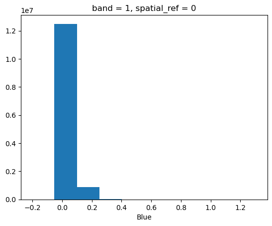
First grab the blue band for the scene

hls_band = rioxarray.open_rasterio(the_tif,mask_and_scale=True)
hls_band = hls_band.squeeze()

33.8.1.1. Now get the transform for Zone 21N

n_tf = hls_band.rio.transform()
print(f"{n_tf.f=}")

n_tf.f=-3799980.0

hls_band.plot.hist();

33.8.2. Change the transform by adding the false northing

We just need to add the northing to the f component and put the pieces back together.

northing = 1.e7  #10 million m
s_tf = affine.Affine(n_tf.a, n_tf.b, n_tf.c, n_tf.d, n_tf.e, n_tf.f + northing)
s_tf

Affine(30.0, 0.0, 300000.0,
       0.0, -30.0, 6200020.0)

33.8.3. Use the modified transform to get the extent for cartopy in the 21S crs

Find the corners like we did in Create the bounding box using the upper left and lower right corners

nrows, ncols = hls_band.rio.shape

ur_x, ur_y = s_tf*(0,0)
lr_x, lr_y = s_tf*(nrows,ncols)

image_extent = [ur_x, lr_x, lr_y, ur_y]

33.9. Use the new make_pal

help(make_pal)

Help on function make_pal in module a301_lib:

make_pal(ax=None, vmin=None, vmax=None, palette='viridis')
    return a dictionary containing a palette and a Normalize object

    Parameters
    ----------

    vmin: minimum colorbar value (optional, defaults to minimum data value)
    vmax: maximum colorbar value (optional, defaults to maximum data value)
    palette: string (optional, defaults to "viridis")

    Returns
    -------

    out_dict: dict
      dictionary with key:values  cmap:colormap, norm:Normalize

vmin = 0.0
vmax = 0.1
pal_dict = make_pal(vmin=vmin,vmax=vmax)
pal_dict

{'cmap': <matplotlib.colors.ListedColormap at 0x129cf1190>,
 'norm': <matplotlib.colors.Normalize at 0x129eca190>}

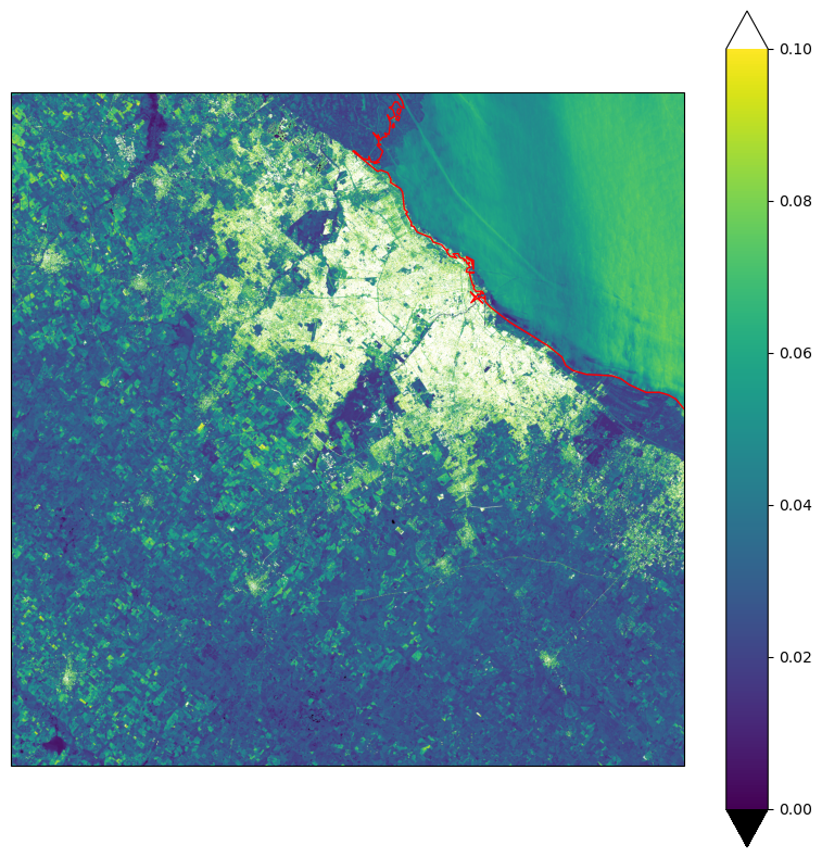
fig, ax = plt.subplots(1, 1, figsize=(10, 10), subplot_kw={"projection": the_crsS})
cs = ax.imshow(
    hls_band.data,
    origin="upper",
    norm = pal_dict['norm'],
    cmap = pal_dict['cmap'],
    extent=image_extent,
    transform=the_crsS
)
ax.add_feature(cartopy.feature.GSHHSFeature(scale="auto", levels=[1, 2, 3],edgecolor='red'))
fig.colorbar(cs,extend='both');