22. Optical depth and partial transmission#
22.1. Notes on optical depth and grey layers#
We need to connect the layer model showing Wallace and Hobbs Figure 4.9 p. 122 with Beer’s law and optical depth.
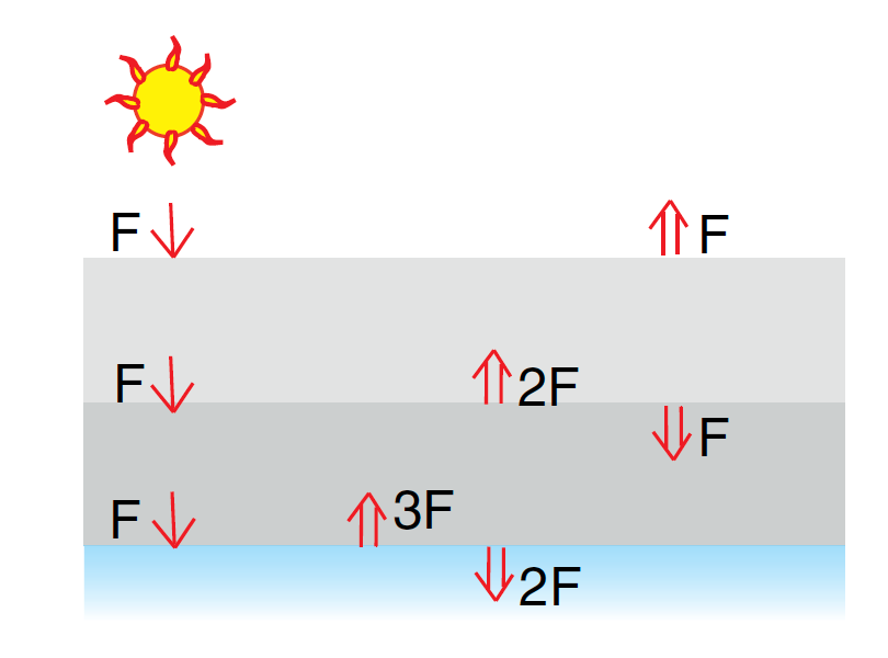
Fig. 22.1 Wallace and Hobbs Figure 4.9: two black layers#
In Fig. 22.1 the absorptivity \(\alpha\) and emissivity \(\epsilon\) are both 1, and the transmissivity \(T\) is 0, because the layers are black. But we know that in general the atmosphere is at least partially transparent in the longwave (we can measure the surface temperature from satellites), so that the flux transmissivity from Week 1 (8.1):
is greater than 0. In fact if we average across all wavelengths and the depth of the atmosphere atmosphere, \(T \approx 0.2\) so \(\epsilon \approx 0.8\))
Wallace and Hobbs make two changes to (22.1):
They use radiance instead of flux
(22.1) only works for “direct beam” flux. Later in the course we’ll see how it has to be modified for the more general case of photons coming from all directions (specifically, we need to get to Wallace and Hobbs equation 4.44 on page 136). Wallace and Hobbs equation 4.17 is always true though:
(22.2)#\[ d I_\lambda=-I_\lambda \rho r k_\lambda d s = -I_\lambda \rho r k_\lambda dz/\cos \theta = -I_\lambda \, d\tau/\cos \theta \]where \(\rho\) is the air density (\(kg\,m^{-3}\)), \(r\) is the gas mixing ratio (kg gas/kg air) and \(k_\lambda\) is the mass absorption coefficient (\(m^{2}\,kg^{-1}\)).
To get the flux equation (22.1) for the direct beam (like the solar beam), just multiply by the small field of view \(\Delta \omega\), since in that case \(F = I \Delta \omega\).
they allow for “slant paths” where the beam is moving at an angle \(\theta\) from the vertical, and so covering a longer distance. For (22.1) we need to limit ourselves to straight up and down with \(\theta = 0\).
22.2. Optical depth and the greybody approximation#
So if the real atmosphere is semi-transparent, how do we modify Fig. 22.1 to be more accurate? We use the “greybody” approximation. If we know the optical depth \(\tau\), then we know the transmissivity \(T = \exp(-\tau)\). If we can neglect reflectivity \(R\) (a good approximation in the longwave), then Wallace and Hobbs equation 4.14 gets simpler:
Conservation of energy:
becomes
where we have used Kirchoff’s law that \(\alpha = \epsilon\). So we’re in a position to calculate absorption and emission for any part of the atmosphere, as long as we know its composition, density and temperature.
22.3. The grey layer in Wallace and Hobbs problem 4.39#
Wallace and Hobbs problem 4.39 describes the folowing grey layer, where I will write the layer temperature as \(T_L\) instead of their \(T^*\):
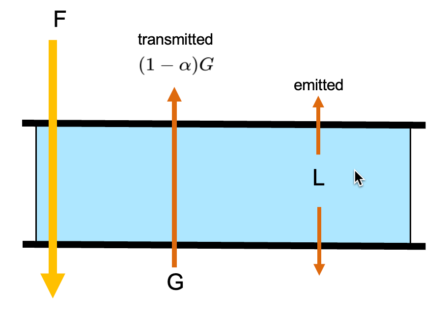
Fig. 22.2 Wallace and Hobbs problem 4.39: A thin grey layer#
Red arrows denote longwave radiation, and the yellow arrow is solar radiation. The arrow labeled \(F\) is the flux arriving from the sun, the unkown arrows are \(L\), the flux emitted by the layer and \(G\) the flux arriving from below the layer. There are two equations because at both the top and bottom of the layer the fluxes have to be exactly equal, or the layer would be heating or cooling. Traditionally, downward arrows are given a positive sign, and negative arrows are given a positive sign. To solve the problem, use the two equations to solve for \(L\) in terms of \(F\) and show that
To get Wallace and Hobbs answer, recognize that the definition of the equilibrium temperature \(T_E\) is the temperature a blackbody would need to balance \(F\), that is:
and by Kirchoff’s law
22.4. Summary#
Given values for gas density, mixing ratio and the absorption coefficient we can compute the optical depth along a path.
Once we know the optical depth, and in the absense of reflection, we can get the transmivity \(T\), the absorptivity \(\alpha\) and the emissivity \(\epsilon\)
We can then use that information to calculate the energy transfer between more realistic atmospheric layers, which will allows us to get the greenhouse effect later in the course.