GOES-16: True Color Images from GOES ABI

43. GOES-16: True Color Images from GOES ABI#

Download the goes_true_color.ipynb notebook from the week8 folder

43.1. Introduction#

This is a modified version of Brian Blaylock’s UCAR python gallery notebook. Blaylock is the author of the GOES download package goes2go used below. I’ve made some changes to the notebook to expand the explanations and fix some bugs caused by changes to the data format and cartopy.

The notebook shows how to make a true color image from the GOES-16 Advanced Baseline Imager (ABI) level 2 data. We will plot the image with matplotlib and Cartopy. The image can be displayed on any map projection after applying a transformation.

Some background: Take a look at the 16 channels described on page 230 of Stull Chapter 8. Note that unlike Modis or Landsat OLI, the ABI doesn’t have a visible channel at green wavelengths, substituting the near-ir 0.846–0.885 \(\mu m\) wavelength range for green. Since that channel is very responsive to plant chlorophyll it’s possible to still use that as part of a proxy for green as shown below. As of March 2025 GOES 18 is GOES West, and GOES 16 is GOES East, with GOES 17 moved into a parking position and GOES 19 ready to replace GOES 16 in Aparil. For more background on GOES, see NOAA’s beginner guide to GOES.

43.1.1. Current GOES satellites#

There are three active GOES satellite on station as of February, 2025. See the NESDIS website for a full list.

GOES 16 is GOES East, parked at -75 degrees West longitude over the equator
GOES 18 is GOES West, parked at -136.9 degrees West longitude
GOES 19 will replace GOES 16 in April, 2025

We will be using the Advanced Baseline Imager Level 2 Cloud and Moisture Product from the Amazon AWS GOES repository. The full list of available GOES products on AWS is here.

The file we’ll download is domain ‘C’ of the “Cloud Moisture Imagery” dataset – abbreviated ABI-L2-MCMIPC which expands to “Advanced Baseline Imager level 2 Cloud Moisture Imagery Product for the Continental US”. It’s about 68 Mbytes, compared to the full disk file (ABI-L2-MCMIPC domain F) which is about 305 Mbytes. A folder called ~/repos/a301/satdata/goes will be created to hold the download.

43.2. Channels and workflow#

These are the channels that contribute to the true-color composite:

–	Wavelength	Channel	Description
Red	0.64 m	2	Red Visible
Green	0.86 m	3	Veggie Near-IR
Blue	0.47 m	1	Blue Visible

The workflow for the notebook:

Find a scene using goes2go
Read the metadata and channels into an xarray dataset
Create the cartopy crs for the scene using the xarray metpy plugin.
Get the original_extent for the image in the geostationary projection crs so we can plot it
Produce a weighted “pseudo-green” image using a weighted combination of the 3 bands to replace the missing green band.
Clip the band values to 0-1 and apply a “gamma correction” (an alternative to the histogram equalization we used in Making color composite (“false color”) images)
Stack the 3 bands in rgb order using numpy depth stacking
Plot the mapped image using cartopy
Zoom the image by changing the axis extent

from goes2go.data import goes_nearesttime
import xarray
from datetime import datetime, timedelta
from pathlib import Path
import cartopy
import numpy as np

import matplotlib.pyplot as plt
import cartopy.crs as ccrs
import cartopy.feature as cfeature
from pathlib import Path
import warnings
warnings.filterwarnings('ignore')

/Users/phil/mini310/envs/a301/lib/python3.13/site-packages/goes2go/data.py:673: FutureWarning: 'H' is deprecated and will be removed in a future version. Please use 'h' instead of 'H'.
  within=pd.to_timedelta(config["nearesttime"].get("within", "1h")),
/Users/phil/mini310/envs/a301/lib/python3.13/site-packages/goes2go/NEW.py:185: FutureWarning: 'H' is deprecated and will be removed in a future version. Please use 'h' instead of 'H'.
  within=pd.to_timedelta(config["nearesttime"].get("within", "1h")),

43.4. Get the x,y extent and start time#

original_extent=(band_2.x.data.min(), band_2.x.data.max(), band_2.y.data.min(), band_2.y.data.max())
original_extent

(np.float64(-3626269.332309611),
 np.float64(1381769.9431296065),
 np.float64(1584175.830644913),
 np.float64(4588197.756226748))

goesC.time_coverage_start

'2020-06-25T18:01:17.2Z'

43.5. Get Date and Time Information#

Each file represents the data collected during one scan sequence for the domain. There are several different time stamps in this file, which are also found in the file’s name.

# Scan's start time, converted to datetime object
scan_start = datetime.strptime(goesC.time_coverage_start, "%Y-%m-%dT%H:%M:%S.%fZ")

# Scan's end time, converted to datetime object
scan_end = datetime.strptime(goesC.time_coverage_end, "%Y-%m-%dT%H:%M:%S.%fZ")

# File creation time, convert to datetime object
file_created = datetime.strptime(goesC.date_created, "%Y-%m-%dT%H:%M:%S.%fZ")
#
# arithmetic on datetime objects
#
duration = (scan_end - scan_start).seconds / 60
midpoint = scan_start + timedelta(minutes = duration/2.)

print(f"Scan Start    : {scan_start}")
print(f"Scan End      : {scan_end}")
print(f"File Created  :  {file_created}")
print(f"Scan midpoint :  {midpoint}")

Scan Start    : 2020-06-25 18:01:17.200000
Scan End      : 2020-06-25 18:03:55.100000
File Created  :  2020-06-25 18:04:10.400000
Scan midpoint :  2020-06-25 18:02:35.700000

43.6. True Color Recipe#

43.6.1. Gamma correction#

Color images are a Red-Green-Blue (RGB) composite of three different channels. We will assign the following channels as our RGB values:

RGB values must be between 0 and 1, same as the range of values of the reflectance channels. A gamma correction is applied to control the brightness and make the image not look too dark, where for input and output values brightness values V the gamma correction is:

(43.1)#\[ V_{out} = V_{in}^{1/\gamma} \]

This correction will enhance the distance between smaller values ov \(V_{in}\) (i.e. more levels for darker colors)

To see why this is, suppose \(\gamma = 2\), so \(1/\gamma\)=0.5. Take the derivative of (43.1):

\[ \frac{dV_{out}}{dV_{in}} = \frac{1}{\gamma V_{in}^{0.5}} \]

so the smaller the magnitude of \(V_{in}\), the larger the difference between \(dV_{out}\) and \(dV_{in}\)

Most displays have a decoding gamma of 2.2. See wikipedia, and this tutorial if you’d like to know more.

43.6.2. Natural vs. veggie green#

The GREEN “veggie” channel on GOES-16 corresponds to the landsat NIR band 5. We could use that channel in place of green, but it would make the green in our image appear too vibrant. Instead, we will tone-down the green channel by interpolating the value to simulate a natural green color.

(43.2)#\[\begin{equation} pseudoGreen = (0.48358168*RED) + (0.06038137*GREEN) + (0.45706946*BLUE) \end{equation}\]

or, a simple alternative (CIMSS Natural True Color):

\[ pseudoGreen = (0.45*RED) + (0.1*GREEN) + (0.45*BLUE) \]

The multiband formatted file we loaded is convenient because all the GOES channels are in the same NetCDF file. Next, we will assign our variables R, G, and B as the data for each channel.

43.8. Clip the bands and apply the gamma correction#

######################################################################
#

# Load the three channels into appropriate R, G, and B variables
R = goesC["CMI_C02"].data
G = goesC["CMI_C03"].data
B = goesC["CMI_C01"].data

######################################################################
#

# Apply range limits for each channel. RGB values must be between 0 and 1
R = np.clip(R, 0, 1)
G = np.clip(G, 0, 1)
B = np.clip(B, 0, 1)

######################################################################
#

# Apply a gamma correction to the image
gamma = 2.2
R = np.power(R, 1 / gamma)
G = np.power(G, 1 / gamma)
B = np.power(B, 1 / gamma)

######################################################################

43.9. Make “true” green from the three bands#

# Calculate the "True" Green
G_true = 0.45 * R + 0.1 * G + 0.45 * B
G_true = np.maximum(G_true, 0)
G_true = np.minimum(G_true, 1)

43.10. Plot the raw images#

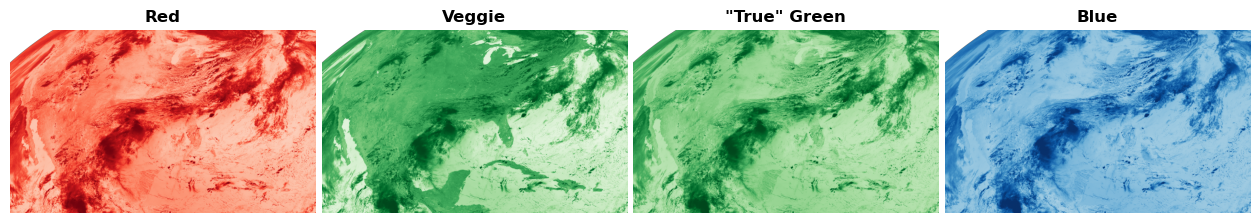
First, we plot each channel individually. The deeper the color means the satellite is observing more light in that channel. Clouds appear white becuase they reflect lots of red, green, and blue light. You will also notice that the land reflects a lot of “green” in the veggie channel becuase this channel is sensitive to the chlorophyll.

fig, ([ax1, ax2, ax3, ax4]) = plt.subplots(1, 4, figsize=(16, 3))

ax1.imshow(R, cmap="Reds", vmax=1, vmin=0)
ax1.set_title("Red", fontweight="semibold")
ax1.axis("off")

ax2.imshow(G, cmap="Greens", vmax=1, vmin=0)
ax2.set_title("Veggie", fontweight="semibold")
ax2.axis("off")

ax3.imshow(G_true, cmap="Greens", vmax=1, vmin=0)
ax3.set_title('"True" Green', fontweight="semibold")
ax3.axis("off")

ax4.imshow(B, cmap="Blues", vmax=1, vmin=0)
ax4.set_title("Blue", fontweight="semibold")
ax4.axis("off")

plt.subplots_adjust(wspace=0.02)

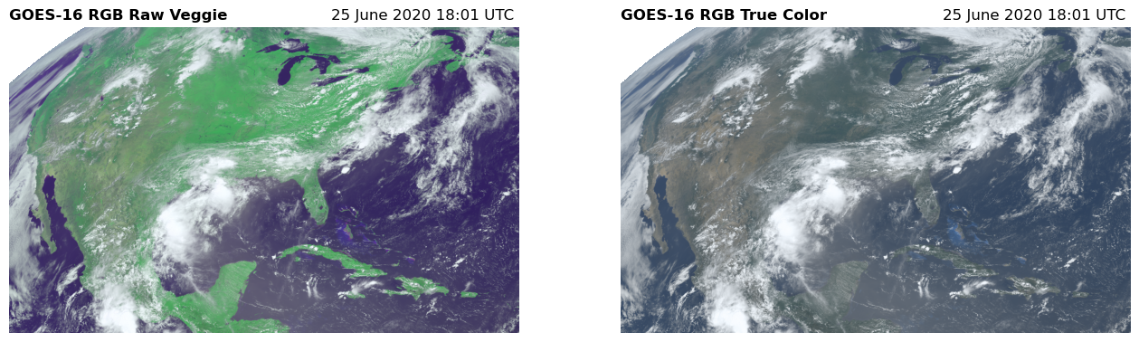
../../_images/ffbc78a518d797fed270d7a16ca6a43ab6282193c8b794a1de4edbee31a39880.png

43.11. Stack the tree images using dstack#

Compare a stack with “veggie green” with “true green” using false color images

######################################################################
# The addition of the three channels results in a color image. We combine the
# three channels in a stacked array and display the image with `imshow` again.
#

# The RGB array with the raw veggie band
RGB_veggie = np.dstack([R, G, B])

# The RGB array for the true color image
RGB = np.dstack([R, G_true, B])

fig, (ax1, ax2) = plt.subplots(1, 2, figsize=(16, 6))

# The RGB using the raw veggie band
ax1.imshow(RGB_veggie)
ax1.set_title("GOES-16 RGB Raw Veggie", fontweight="semibold", loc="left", fontsize=12)
ax1.set_title("%s" % scan_start.strftime("%d %B %Y %H:%M UTC "), loc="right")
ax1.axis("off")

# The RGB for the true color image
ax2.imshow(RGB)
ax2.set_title("GOES-16 RGB True Color", fontweight="semibold", loc="left", fontsize=12)
ax2.set_title("%s" % scan_start.strftime("%d %B %Y %H:%M UTC "), loc="right")
ax2.axis("off");

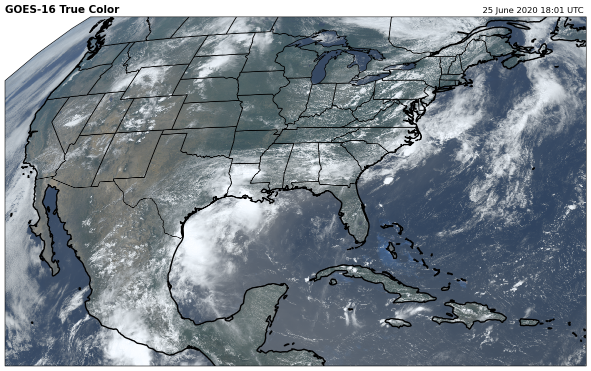
../../_images/b967c08e6a0cc779eead2cbdfcdc09173e6cbdff5035d3e4a722149550a5c8f9.png

43.12. Plot the mapped image using cartopy#

fig = plt.figure(figsize=(15, 12))

ax = fig.add_subplot(1, 1, 1, projection=cartopy_crs)

ax.imshow(
    RGB,
    origin="upper",
    extent= original_extent,
    transform=cartopy_crs,
    interpolation="nearest",
    vmin=162.0,
    vmax=330.0,
)
ax.coastlines(resolution="50m", color="black", linewidth=2)
ax.add_feature(ccrs.cartopy.feature.STATES)

plt.title("GOES-16 True Color", loc="left", fontweight="semibold", fontsize=15)
plt.title("%s" % scan_start.strftime("%d %B %Y %H:%M UTC "), loc="right");

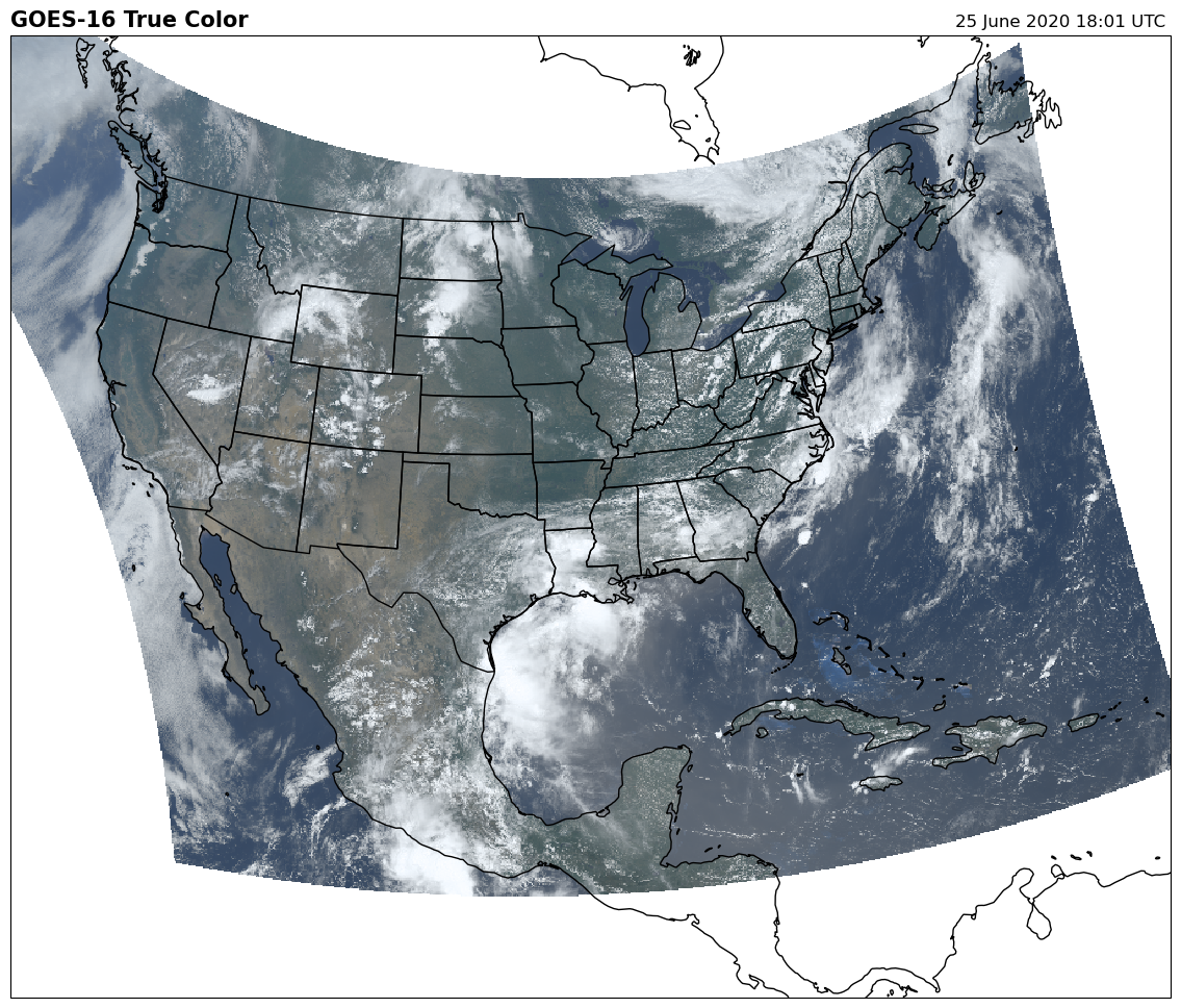
../../_images/5dbbc925f93f83d1c76232490c4fdf0a5b8856501e6cbbff5cab78363cb1427f.png

43.13. Changing the map projection and plot extent#

The next two cells show how to change the plotting crs and boundaries (extent) on a plot

The plot below changes the crs to LambertConformal and sets the plotting extent to between -130- -60 deg lon and 10 - 65 deg lat

fig = plt.figure(figsize=(15, 12))

lc = ccrs.LambertConformal(central_longitude=-97.5)
#
# add an axiss with the lc projection
#
ax = fig.add_subplot(1, 1, 1, projection=lc)
#
# lat/lons are given in "flat-square" projection
#
ax.set_extent([-120, -65, 10, 55], crs=ccrs.PlateCarree())

ax.imshow(
    RGB,
    origin="upper",
    extent=original_extent,
    transform=cartopy_crs,
    interpolation="none",
)
ax.coastlines(resolution="50m", color="black", linewidth=1)
ax.add_feature(ccrs.cartopy.feature.STATES)

plt.title("GOES-16 True Color", loc="left", fontweight="semibold", fontsize=15)
plt.title("%s" % scan_start.strftime("%d %B %Y %H:%M UTC "), loc="right");

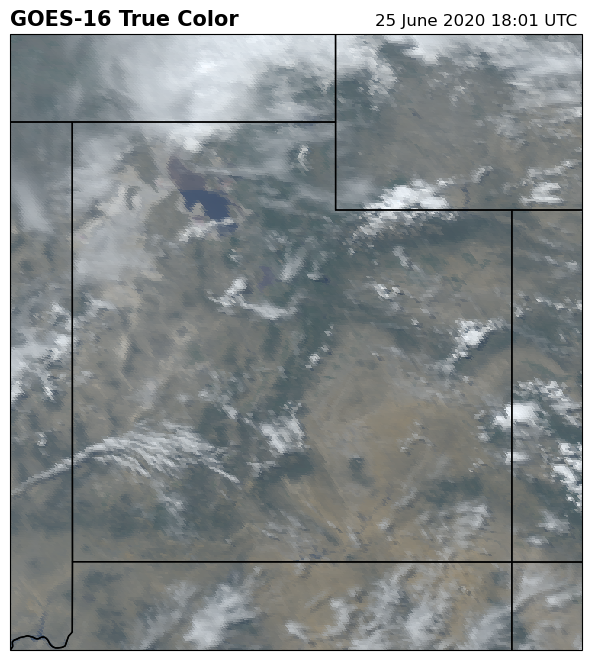
../../_images/793536d503f792d7e094d0dc32ba2aba23ac1a1c6a3927d6951b7ab0bdb5bc19.png

43.14. Change the axis extent (not the original image extent)#

We can zoom the map to a lon/lat box by specifying a new extent for the axis between -114.5 - -108.25 deg Lon and 36-43 deg Lat – Salt Lake City, Utah The axis crs is switched to PlateCarree, which is ok at this small scale (where the lat/lon parallels are basically straight lines)

fig = plt.figure(figsize=(8, 8))

#
# GOES 
#
pc = ccrs.PlateCarree()

ax = fig.add_subplot(1, 1, 1, projection=pc)
#
# utah
#
ax.set_extent([-114.75, -108.25, 36, 43], crs=pc)

ax.imshow(RGB, 
          origin='upper',
          extent=original_extent,
          transform=cartopy_crs,
          interpolation='none')

ax.coastlines(resolution='50m', color='black', linewidth=1)
ax.add_feature(ccrs.cartopy.feature.STATES)

plt.title('GOES-16 True Color', loc='left', fontweight='bold', fontsize=15)
plt.title('{}'.format(scan_start.strftime('%d %B %Y %H:%M UTC ')), loc='right');

../../_images/22920ba49f96012a1150306f3accc8d3a583ab5f3c7f802aeaaed3b587eabc11.png

43.15. Practice questions (takehome exam prep)#

43.15.1. Practice question 1#

Use a seaborn jointplot to compare the channel 1 (blue) histogram before and after the gamma correction

43.15.2. Practice question 2#

Use xarray.isel to clip just the portion of the abi scene that’s in the [-114.75, -108.25, 36, 43] lon/lat bounding box and save it to disk as a netcdf file with the correct affine transform and crs

43.15.3. Practice question 3#

Change the map projection in from lambert to azimuthal equal area – does it look less weird?

43.15.4. Practice question 4#

Write a channel out as a geotiff file by first converting it to a rioxarray

43.15.5. Pratice question 5#

Use the full domain image to produce a picture of a region in the southern hemisphere or Canada